[-] Contents
Hilbert, in his 9th problem, posed the problem of finding the general reciprocity law for any number field. The class field theory developed in the first half of the 20th century was successful in answering this question for finite abelian extensions of  . As an easy consequence of class field theory, one can reproduce the classical Kronecker-Weber theorem, that is, every finite abelian extension of is a subfield of some cyclotomic extension
  of . Hilbert's 12th problem also asked how to extend the Kronecker-Weber theorem to an arbitrary ground number field, in other words, how to describe abelian extensions of a number field more explicitly.
Motivated by the case of where all abelian extensions are obtained by adjoining the values of the exponential function, Kronecker conjectured, while he was studying elliptic functions, that all abelian extensions of an imaginary quadratic field should also arise in such a manner. This was achieved by the beautiful theory of complex multiplication, which allows one to describe all abelian extensions of an imaginary quadratic field via the values of the modular  -function and the Weber function, or in the language of elliptic curves, via the -invariant and (certain powers of)
  -coordinates of all torsion points of the corresponding elliptic curve. This problem for general number fields, known as Kronecker's Jugendtraum (dream of youth), is still largely open and is at the heart of current research in number theory.
In this chapter, we will start by establishing the one-one correspondence between  , the ideal class group of an order
  in an imaginary quadratic field
  , and
, and  , the set of all isomorphism classes of elliptic curves with complex multiplication by . Next, we will define the ring class field of and then prove that it is obtained by adjoining the value
  for any proper fractional ideal of , using the method of reduction of elliptic curves. Moreover, the ray class fields of can be obtained by adjoining the values of the Weber function. Next, we will discuss the modular equation and use it to prove the integrality of . The values of , i.e., the values of
  at the imaginary quadratic argument
  , are called singular moduli as they correspond to the -invariants of singular elliptic curves. We will use Weber's method to explicitly compute singular moduli for orders of class number 1. These singular moduli turn out to be highly divisible as predicted by a remarkable theorem of Gross and Zagier. Gross and Zagier's theorem on singular moduli completely determines the prime factorization of the norm of the difference between two singular moduli. Our last section will be devoted to the algebraic proof of this theorem, relying on Deuring's results on the endomorphism rings of elliptic curves.
 Complex multiplication
As we saw in the first chapter, for a complex elliptic curve  , the endomorphism ring
  can be identified with
  . When
  has complex multiplication, is an order in an imaginary quadratic extension of . Though complex conjugation will give us two isomorphisms between and
  , we do have a canonical way to identify with . Namely, for every
  , we identify it with the endomorphism
 ![$[\alpha]$](./latex/latex2png-MinorThesis3_68781034_-5.gif) of induced by the multiplication
of induced by the multiplication  . In other words, the effect of on the invariant differential is given by
 ![$[\alpha]^*\omega=\alpha\cdot\omega$](./latex/latex2png-MinorThesis3_191623990_-5.gif) . We call this identification the normalized identification.
. We call this identification the normalized identification.
Example 1
Let  , then
  ,
,  and has complex multiplication by
 ![$\mathbb{Z}[i]$](./latex/latex2png-MinorThesis3_42772926_-5.gif) . The normalized identification is given by the endomorphism
. The normalized identification is given by the endomorphism =(-x,iy)$](./latex/latex2png-MinorThesis3_140351950_-5.gif) , since
, since ![$[i]^*(dx/y)=d(-x)/(iy)=i(dx/y)$](./latex/latex2png-MinorThesis3_63969329_-5.gif) .
.
, then , and has complex multiplication by . The normalized identification is given by the endomorphism , since .
Example 2
Let  , then
  ,
,  and has complex multiplication by
 ![$\mathbb{Z}[\rho]$](./latex/latex2png-MinorThesis3_49444867_-5.gif) , where
, where  . The normalized identification is given by the endomorphism
 =(\rho x,y)$](./latex/latex2png-MinorThesis3_99374539_-5.gif) , since
, since ![$[\rho]^*(dx/y)=d(\rho x)/y=\rho(dx/y)$](./latex/latex2png-MinorThesis3_148630286_-5.gif) .
.
, then , and has complex multiplication by , where . The normalized identification is given by the endomorphism , since .
Fix an order in . We are interested in studying all complex elliptic curves with endomorphism ring . We denote the set of all these isomorphism classes by . As we will see in Theorem 1, it turns out that is in bijection with a purely algebraic object constructed from , namely the ideal class group of .
Definition 1
Let and be as above. Let  be a fractional ideal of , then
  is a ring and contains the order , so it is also an order. We say that is proper if is equal to .
and be as above. Let be a fractional ideal of , then is a ring and contains the order , so it is also an order. We say that is proper if is equal to .
Definition 2
The set of all proper fractional ideals of , denoted by  , forms a group ([1, 4.11]), called the ideal group of . Denote by
  the subgroup of principal proper fractional ideals. The quotient group
  is called the ideal class group of . When is the ring of integers
  , we recover the ideal class group of in the usual sense.
, denoted by , forms a group ([1, 4.11]), called the ideal group of . Denote by the subgroup of principal proper fractional ideals. The quotient group is called the ideal class group of . When is the ring of integers , we recover the ideal class group of in the usual sense.
Remark 1
A fractional ideal of is proper if and only if it is locally principal ([1, 5.4.2]), hence can be viewed as the reduced Grothendieck group  , i.e., the group of projective -modules of rank 1 ([2]).
is proper if and only if it is locally principal ([1, 5.4.2]), hence can be viewed as the reduced Grothendieck group , i.e., the group of projective -modules of rank 1 ([2]).
Theorem 1
Let be a complex elliptic curve with  , then
  for some proper fractional ideal of . Moreover,
  if and only and
  are in the same ideal class. Conversely, for every proper fractional ideal ,
  .
.
be a complex elliptic curve with , then for some proper fractional ideal of . Moreover, if and only and are in the same ideal class. Conversely, for every proper fractional ideal , .
In other words, the above correspondence gives a bijection  .
.
Proof
Since is a complex elliptic curve, by Example 1 we know that  for some lattice
  for some
  . We can view
  as a fractional ideal of . Then, under the normalized identification,
  Therefore is a proper fractional ideal. Moreover, if and only if
  for some
  , if and only if and are in the same ideal class, since every principal fractional ideal is automatically proper.
is a complex elliptic curve, by Example 1 we know that for some lattice for some . We can view as a fractional ideal of . Then, under the normalized identification, Therefore is a proper fractional ideal. Moreover, if and only if for some , if and only if and are in the same ideal class, since every principal fractional ideal is automatically proper.
Conversely, suppose is a proper fractional ideal, then  , hence .
□
, hence .
□
We will soon see that is a finite group. The order of , denoted by  , is called the class number of . So by Theorem 1, there are exactly isomorphism classes of elliptic curves with complex multiplication by and each of them corresponds to an ideal class of . Let be an elliptic curve with , then for any automorphism
  of
of  ,
,  is also an elliptic curve with . So by the finiteness of the ideal class group and the above correspondence between and , we know
  has finitely many values, hence
  is an algebraic number of degree at most
  .
.
An amazing fact is that for an elliptic curve with complex multiplication by , is actually an algebraic integer of degree (Theorem 8). In particular, an elliptic curve with complex multiplication has a rational -invariant if and only  . We will calculate these -invariants later.
Ring class fields
Let be an imaginary quadratic extension of of discriminant  . The ring of integers of is equal to
  where
where  . Every order of is a free
  -module of rank 2, hence is of the form
  , where the positive integer
  is called the conductor of . When
  ,
,  is the maximal order and is a Dedekind domain. But when
  , is not integrally closed and hence is not a Dedekind domain. So it is not necessary for the unique factorization to hold for ideals in . For example,
 ![${\cal O}=\mathbb{Z}[\sqrt{-3}]$](./latex/latex2png-MinorThesis3_181885576_-5.gif) is an order of conductor 2 of
is an order of conductor 2 of  , and the ideal
  has two different prime factorizations
  . However, we will see that the situation becomes better when we restrict our attention to the ideals prime to .
Proposition 1
Every ideal of prime to is proper. An ideal of is prime to if and only if  is prime to .
prime to is proper. An ideal of is prime to if and only if is prime to .
Proof
Suppose is an ideal of prime to . By definition,  . Suppose
  such that
  , then
  Hence
Hence  . It follows that is proper.
is an ideal of prime to . By definition, . Suppose such that , then Hence . It follows that is proper.
Next, let  be multiplication by . Then
  if and only if
  is surjective. But
  is an finite abelian group of order , so is surjective if and only if is prime to .
□
is an finite abelian group of order , so is surjective if and only if is prime to .
□
Therefore the ideals prime to are in and are closed under multiplication. They generate a subgroup of fractional ideals  . Similarly define
  . Given any integer , every ideal class in contains an ideal prime to ([3, 7.17]). So the natural inclusion induces a surjective map
  . Moreover, the kernel of this surjective map is , so we have an isomorphism
  ([3, 7.19]).
Since is a Dedekind domain, the first part of the next Proposition 2 ([3, 7.20, 7.22]) tells us that unique factorization does hold for fractional ideals of prime to .
Proposition 2
The map  induces an isomorphism
  , and the inverse map is given by
  . The isomorphism induces an isomorphism
  , where
induces an isomorphism , and the inverse map is given by . The isomorphism induces an isomorphism , where
Viewing as a cycle of , we know that  and that
  is a subgroup of
  containing
  (we use the symbols for generalized ideal groups as in [4, VI]). Hence, by class field theory, corresponds to a finite abelian extension
  of .
of .
 is called the ring class field of
 Combining the isomorphism and the second part of Proposition 2, we know that  , and composing with the Artin map we obtain an isomorphism
  . In particular, is a finite group. Again, when , i.e., is the maximal order , the ring class field of is just the usual Hilbert class field of . So we may regard the ring class field as a generalization of the Hilbert class field.
Remark 2
The ring class field of the order ![$\mathbb{Z}[-\sqrt{n}]$](./latex/latex2png-MinorThesis3_136031181_-5.gif) is related to the classical problem of determining the primes of the form
is related to the classical problem of determining the primes of the form  studied by Fermat, Euler, Lagrange, Legendre and Gauss. More precisely, let
  be a real algebraic integer such that the ring class field
  and let
  be its minimal polynomial, then for odd
  dividing neither
  nor the discriminant of , we have
  See [3] for this beautiful story.
is related to the classical problem of determining the primes of the form studied by Fermat, Euler, Lagrange, Legendre and Gauss. More precisely, let be a real algebraic integer such that the ring class field and let be its minimal polynomial, then for odd dividing neither nor the discriminant of , we have See [3] for this beautiful story.
Main theorems of complex multiplication
The first main result of this section is the ``First Main Theorem'' of complex multiplication, which says the ring class field of can be obtained by adjoining the value of -function at any proper ideal of . The key step of the proof is to establish the so-called Hasse congruence (Theorem 2), which expresses the Frobenius action on the value of the -function via the action on the argument of the -function. There are several different approaches to do so: the complex analytic method using the modular equation, or the algebraic method we choose here using the reduction of elliptic curves. We follow mainly the exposition of [5] and [3].
First, by using Chebotarev's density theorem, one can show the following characterization of field extensions by the primes which split completely ([3, 8.20]). We will utilize this Lemma 1 twice to characterize the ring class field in Lemma 2.
Lemma 1
Let be a number field. Let  be a finite Galois extension of and
  be a finite extension of . Then
  if and only if for all but finitely many unramified primes
  of which have a degree 1 prime
  of above , splits completely in .
be a number field. Let be a finite Galois extension of and be a finite extension of . Then if and only if for all but finitely many unramified primes of which have a degree 1 prime of above , splits completely in .
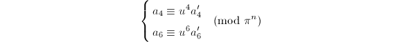
From now on, let us fix an order of conductor in an imaginary quadratic field . Let  (
( ) be the representatives of the ideal class group and
  be the corresponding elliptic curves with complex multiplication by via Theorem 1. Let
 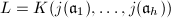 .
.
Lemma 2
Let be a prime which splits as  . If for all but finitely many such , we have the congruence
  for any proper fractional ideal of and any prime of over , then is the ring class field of for any proper fractional ideal of .
be a prime which splits as . If for all but finitely many such , we have the congruence for any proper fractional ideal of and any prime of over , then is the ring class field of for any proper fractional ideal of .
Proof
Let be the ring class field of . Let us first show that  . Suppose is a unramified prime of and is a degree 1 prime of over . By Lemma 1, it suffices to show that for all but finitely many such , splits completely in . Since is of degree 1, we already know that must split completely as in for some primes
  of . By the assumption, for all but finitely many such , we have
  where the second equality is because has degree 1. Excluding the finitely many primes such that divides any of the differences
  , we conclude that
  for all but finitely many primes . So is a principal ideal of and hence has trivial Artin symbol, therefore splits completely in .
be the ring class field of . Let us first show that . Suppose is a unramified prime of and is a degree 1 prime of over . By Lemma 1, it suffices to show that for all but finitely many such , splits completely in . Since is of degree 1, we already know that must split completely as in for some primes of . By the assumption, for all but finitely many such , we have where the second equality is because has degree 1. Excluding the finitely many primes such that divides any of the differences , we conclude that for all but finitely many primes . So is a principal ideal of and hence has trivial Artin symbol, therefore splits completely in .
Next let us show that  . Let be the Galois closure of . Suppose is a prime which splits completely in . Again by Lemma 1, it suffices to show that for all but finitely such , splits completely in . Since splits completely in , must be a principal ideal of and then
  . So by assumption,
  for all but finitely many such and any prime of above . Now suppose further that does not divide the index
 ![$[{\cal O}_L:{\cal O}_K(j(\mathfrak{a}))]$](./latex/latex2png-MinorThesis3_72240984_-5.gif) , then we have
, then we have  for any
  , hence has degree 1 for any above . Therefore splits completely in .
□
, hence has degree 1 for any above . Therefore splits completely in .
□
Theorem 2
Let be a prime satisfying that  , splits as and the
  's have good reduction at . Then for any proper fractional ideal of and any prime of above , we have the Hasse congruence
be a prime satisfying that , splits as and the 's have good reduction at . Then for any proper fractional ideal of and any prime of above , we have the Hasse congruence
Proof
Since , and  are proper. We may assume that
  and
and  represent and
  in the ideal classes. Then
  ,
,  and we have a natural isogeny
  since
since  . Because splits completely, we know that
  . Now find an ideal prime to in the ideal class of , then
  is a principal ideal generated by some
  . Therefore
  induces an isogeny
  and
and  is prime to by our choice of . The composition
  is given by
  via the normalized identification of and
  .
.
, and are proper. We may assume that and represent and in the ideal classes. Then , and we have a natural isogeny since . Because splits completely, we know that . Now find an ideal prime to in the ideal class of , then is a principal ideal generated by some . Therefore induces an isogeny and is prime to by our choice of . The composition is given by via the normalized identification of and .
Now since the 's have good reduction at , reducing modulo we get an isogeny 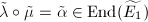 . But , so
  where
where  is the invariant differential of
  . Therefore
  is inseparable. As the reduction does not change the degree of an isogeny,
  is prime to , hence
  is separable. We conclude that
  is inseparable. But
  , hence is purely inseparable. So is the composition of the -Frobenius
  and an isomorphism
  . Hence
  and the claim follows.
□
and the claim follows.
□
From Theorem 2 and Lemma 2, we already know that  is actually the ring class field of . Further more, we can use the limited information of the Hasse congruence to compute the Galois action on the -values.
Theorem 3
For any proper fractional ideal of and  , we have
  for any proper ideal
  , where
  is a prime of whose Artin symbol is . In particular,
  is the Galois orbit of for any proper fractional ideal of and
 ![$[\mathbb{Q}(j(\mathfrak{a})):\mathbb{Q}]=[K(j(\mathfrak{a})):K]=h$](./latex/latex2png-MinorThesis3_141025169_-5.gif) , where .
, where .
of and , we have for any proper ideal , where is a prime of whose Artin symbol is . In particular, is the Galois orbit of for any proper fractional ideal of and , where .
Proof
By Chebotarev's density theorem, there are infinite many degree 1 primes of whose Artin symbol is . By Theorem 2, for all but finitely many such primes (excluding those not prime to ), we have  where is proper and is any prime of over . Since these 's have the same Artin symbol, they must lie in the same ideal class of . So
  is the same for every and has infinitely many prime factors, therefore it must be zero. We conclude that
  . The remaining part follows since
 ![$[K:\mathbb{Q}]\le2$](./latex/latex2png-MinorThesis3_169673901_-5.gif) and we already know
and we already know ![$[\mathbb{Q}(j(\mathfrak{a})):\mathbb{Q}]\le h$](./latex/latex2png-MinorThesis3_232645048_-5.gif) .
□
.
□
of whose Artin symbol is . By Theorem 2, for all but finitely many such primes (excluding those not prime to ), we have where is proper and is any prime of over . Since these 's have the same Artin symbol, they must lie in the same ideal class of . So is the same for every and has infinitely many prime factors, therefore it must be zero. We conclude that . The remaining part follows since and we already know .
□
Now we are in a position to prove the First Main Theorem of complex multiplication.
Theorem 4 (First Main Theorem)
 is the ring class field of for any proper fractional ideal of . In particular,
  is the Hilbert class field of .
is the ring class field of for any proper fractional ideal of . In particular, is the Hilbert class field of .
 as in Remark
 As a consequence of the First Main Theorem 4, all everywhere unramified extensions of can be obtained as a subfield of . Moreover, one can show that an abelian extension of is generalized dihedral over if and only if it is contained in the ring class field of some order in ([3, 9.18]), so the First Main Theorem also tells us how to construct generalized dihedral extensions explicitly. Now, it is natural to ask how to generate all abelian extensions of , in other words, how to give an explicit description of the ray class fields of . This is the content of the ``Second Main Theorem'' of complex multiplication.
Definition 4
Let be an elliptic curve with a Weierstrass model  . For any
  , define the Weber function
 So the Weber function is essentially the -coordinate function on the elliptic curve . Notice that the powers of the coordinate
  and the normalized constants appearing in the expression are chosen in the way that
  is invariant under the isomorphisms of elliptic curves. In the language of lattices, we may define the Weber function
  as follows:
be an elliptic curve with a Weierstrass model . For any , define the Weber function
So the Weber function is essentially the -coordinate function on the elliptic curve . Notice that the powers of the coordinate and the normalized constants appearing in the expression are chosen in the way that is invariant under the isomorphisms of elliptic curves. In the language of lattices, we may define the Weber function as follows:
Now let us establish an analog of the Hasse congruence for the Weber function.
Theorem 5
Let  and be an extension of containing all
  's and
  's. Let be a prime satisfying , splits as and 's have good reduction at . Then for any proper fractional ideal of and any prime of above , we have the congruence
and be an extension of containing all 's and 's. Let be a prime satisfying , splits as and 's have good reduction at . Then for any proper fractional ideal of and any prime of above , we have the congruence
Proof
We proceed as the proof of Theorem 2 and obtain an isogeny  which is the composition of the -Frobenius
  and an isomorphism
  . Since the Weber function is invariant under isomorphisms, we know that
  and the claim follows since
  is just the natural projection.
□
is just the natural projection.
□
which is the composition of the -Frobenius and an isomorphism . Since the Weber function is invariant under isomorphisms, we know that and the claim follows since is just the natural projection.
□
After the congruence in Theorem 5 is established, a similar argument as for ring class fields will allow us to construct all the ray class fields of . We state this Second Main Theorem and omit the details of the proof here. Roughly speaking, the maximal abelian extension of is generated by  and the -coordinates of all torsion points of the corresponding elliptic curve with complex multiplication by . See [3, 11.39] and [6, II.5] for more.
Theorem 6 (Second Main Theorem)
Let be an ideal of and be an elliptic curve with complex multiplication by . Let ![$E[\mathfrak{a}]=\{P\in E\mid [\alpha]P=O, \alpha\in \mathfrak{a}\}$](./latex/latex2png-MinorThesis3_209562922_-5.gif) be the -torsion points of , then
be the -torsion points of , then ![$K(j(E), h(E[\mathfrak{a}],E))$](./latex/latex2png-MinorThesis3_90976662_-5.gif) is the ray class field of with respect to the cycle . In particular, the maximal abelian extension of is equal to
is the ray class field of with respect to the cycle . In particular, the maximal abelian extension of is equal to  .
.
be an ideal of and be an elliptic curve with complex multiplication by . Let be the -torsion points of , then is the ray class field of with respect to the cycle . In particular, the maximal abelian extension of is equal to .
Modular equations and the integrality of singular moduli
We have seen that is an algebraic number of degree from Theorem 3. But in fact more is true: it is an algebraic integer. There are several possible proofs of this fact: the complex analytic proof using the modular equation, the good reduction proof due to Serre and Tate, and the bad reduction proof due to Serre ([6, II.6]). We have not talked much about the analytic aspect of -function so far, so we will choose the first approach here.
Let us first recall some facts about the modular curve  , which plays an important role in modern number theory. The modular curve is a compact Riemann surface constructed by compactifying
  , the quotient of upper half plane by the congruence group
  . It is the compactification of the moduli space of elliptic curves along with the level structure of a cyclic subgroup of order
  . Viewing as a complex algebraic curve, the function field of is equal to
 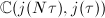 . So has a planar model defined by some complex polynomial
  satisfying
  , called the modular equation of level ([7]).
An unexpected result is that the modular equation in fact has rational, or even better, integer coefficients. Therefore, can be defined as an algebraic curve over without reference to the complex numbers and it has a planar model over defined by the modular equation. The goal of this section is to prove this unexpected fact and deduce the integrality of as a consequence.
To define the modular equation, we need the following lemma.
Lemma 3 (Hasse  -expansion principle)
Let
-expansion principle)
Let  be a modular function with respect to
  with the -expansion
  . Then can be expressed as a polynomial of degree in
 ![$\mathbb{Z}[c_{-t},\ldots,c_0][j(\tau)]$](./latex/latex2png-MinorThesis3_5303128_-5.gif) . In particular, if
. In particular, if  's are integers, then this polynomial has integer coefficients.
-expansion principle)
Let be a modular function with respect to with the -expansion . Then can be expressed as a polynomial of degree in . In particular, if 's are integers, then this polynomial has integer coefficients.
Proof
The proof is by induction on . When  , is a holomorphic function on the compact Riemann surface
  , hence it must be the constant
  . When
  , since has -expansion
  with integer coefficients, the leading term of the -expansion of
  is
is  and all the coefficients are in
 ![$\mathbb{Z}[c_{1-t},\ldots,c_0]$](./latex/latex2png-MinorThesis3_73701902_-5.gif) . Now applying the induction hypothesis, we know
. Now applying the induction hypothesis, we know ![$f-c_{-t}j^t\in \mathbb{Z}[c_{1-t},\ldots,c_0][j]$](./latex/latex2png-MinorThesis3_102709107_-5.gif) is a polynomial of degree
is a polynomial of degree  . The lemma follows.
□
. The lemma follows.
□
. When , is a holomorphic function on the compact Riemann surface , hence it must be the constant . When , since has -expansion with integer coefficients, the leading term of the -expansion of is and all the coefficients are in . Now applying the induction hypothesis, we know is a polynomial of degree . The lemma follows.
□
Definition 5
Let  Suppose
  is a set of orbit representatives for the left action of on
  . We define
  Then the coefficients of
  in
in  are modular functions of , hence by Lemma 3, these coefficients of are polynomials in . So
  is a polynomial, called the modular polynomial or the modular equation of level .
Suppose is a set of orbit representatives for the left action of on . We define Then the coefficients of in are modular functions of , hence by Lemma 3, these coefficients of are polynomials in . So is a polynomial, called the modular polynomial or the modular equation of level .
Since  , it follows immediately that . Also, it is an easy computation ([5, 4.5]) to see that the set of orbit representatives can be chosen as
Theorem 7
The modular equation ![$\Phi_N(X, Y)\in\mathbb{Z}[X, Y]$](./latex/latex2png-MinorThesis3_139773853_-5.gif) . Moreover, when is not a perfect square, the leading coefficient of
. Moreover, when is not a perfect square, the leading coefficient of  is
is  .
.
. Moreover, when is not a perfect square, the leading coefficient of is .
Proof
By Lemma 3, to show , it suffices to show that the -expansions of have integer coefficients. Using the orbit representatives in  , we find that for
  ,
,
 has a Fourier expansion in
  with coefficients in
 ![$\mathbb{Z}[\xi]$](./latex/latex2png-MinorThesis3_128867247_-5.gif) where
where  , hence the coefficients of -expansions of
  are in . For an integer
  prime to , the map
  is a permutation of , hence it leaves unchanged. But this map has an action
  on the coefficients, therefore the coefficients are actually in . So
 ![$\Phi_N(X, Y)\in\mathbb{Z}[X,Y]$](./latex/latex2png-MinorThesis3_65681078_-5.gif) .
.
, it suffices to show that the -expansions of have integer coefficients. Using the orbit representatives in , we find that for ,
has a Fourier expansion in with coefficients in where , hence the coefficients of -expansions of are in . For an integer prime to , the map is a permutation of , hence it leaves unchanged. But this map has an action on the coefficients, therefore the coefficients are actually in . So .
Now suppose is not a perfect square. The leading coefficient of is the same as the leading coefficient of the -expansion of  , so let us show that the latter is . Now begins with
  and begins with
  , so since is not a perfect square and
  , we know that and cannot cancel out, hence the leading coefficient of
  is a root of unity. Multiplying them together, we know that the leading coefficient of
 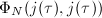 is a root of unity. But we already know it is an integer, hence it must be .
□
is a root of unity. But we already know it is an integer, hence it must be .
□
Example 3
The first two modular equations are computed as
 See [3, 13.B] for an algorithm of computing the modular equations. However, it is usually cumbersome to do the computation even for small levels. The
  case was computed by Smith in 1878; the
  case was computed by Berwick in 1916; the
  case was computed by Herrmann in 1974 and the
  case was computed by Kaltofen and Yui using MACSYMA in 1984. The resulting polynomial
  is of degree 21 with coefficients up to
  and needs 5 pages to be written out.
See [3, 13.B] for an algorithm of computing the modular equations. However, it is usually cumbersome to do the computation even for small levels. The case was computed by Smith in 1878; the case was computed by Berwick in 1916; the case was computed by Herrmann in 1974 and the case was computed by Kaltofen and Yui using MACSYMA in 1984. The resulting polynomial is of degree 21 with coefficients up to and needs 5 pages to be written out.
Now we are in a position to prove the integrality of the singular moduli.
Theorem 8
Let be an order in an imaginary quadratic field and be a proper fractional ideal of . Then is an algebraic integer of degree .
be an order in an imaginary quadratic field and be a proper fractional ideal of . Then is an algebraic integer of degree .
Proof
By Chebotarev's density theorem, there are infinitely many degree 1 primes of in the principal ideal class. Let be such a prime. Then  where
where  is a prime. We may assume that
  , then is homothetic to
  for some
  ([3, 11.24]). We know that
  by definition. But by our choice of . Hence by Theorem 7, satisfies the polynomial
 ![$\Phi_p(X,X)\in\mathbb{Z}[X]$](./latex/latex2png-MinorThesis3_237581038_-5.gif) with leading coefficient and therefore is an algebraic integer. Moreover, we know that its degree is from Theorem 3.
□
with leading coefficient and therefore is an algebraic integer. Moreover, we know that its degree is from Theorem 3.
□
in the principal ideal class. Let be such a prime. Then where is a prime. We may assume that , then is homothetic to for some ([3, 11.24]). We know that by definition. But by our choice of . Hence by Theorem 7, satisfies the polynomial with leading coefficient and therefore is an algebraic integer. Moreover, we know that its degree is from Theorem 3.
□
Weber's computation of singular moduli
As an application of Proposition 2, we get an exact sequence  Hence the class numbers of and are related by
  One can show that there is an exact sequence ([3, Exercise 7.30])
  Therefore we are able to reproduce the following formula due to Gauss for the class number of an order in ([3, 7.24]).
![$$h({\cal O})=\frac{h({\cal O}_K)f}{[{\cal O}_K^*:{\cal O}^*]}\prod_{p\mid f}\left(1-\legendre{d_K}{p}\frac{1}{p}\right).$$](./latex/latex2png-MinorThesis3_215696511_.gif)
Our goal in this section is to compute the  for the orders of class number 1. By Theorem 8, all these singular moduli are rational integers. A famous result about the Gauss class number problem, now known as the Stark-Heegner theorem, says that there only 9 imaginary quadratic fields having class number 1. Moreover, using Theorem 9, we can conclude that there are only four more cases for non-maximal orders of class number 1. More precisely, when
  , only
  and
and  can occur; when
  (i.e.,
  ), only can occur; when
  (i.e.,
  ), only
  can occur. Since an order is uniquely determined by its discriminant
  , we may summarize the results as the following theorem.
Theorem 10
There are only 9 imaginary quadratic fields of class number 1. Their discriminants are  There are only 13 orders of class number 1. Their discriminants are
of class number 1. Their discriminants are
There are only 13 orders of class number 1. Their discriminants are
To compute these singular moduli, one may proceed by plugging into the -expansion of ,  This -expansion can be computed via the -expansions of
  and
and  ,
,  So nowadays we can handle this task using a computer. The numerical method will work pretty well for our purpose since we know a priori that these values are integers. All the 13 singular moduli of integer values are listed in Table 1.
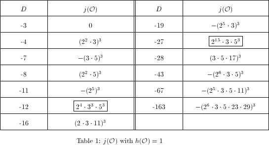
By Theorem 10, we easily obtain a quick method of detecting complex multiplication for elliptic curves over : if appears in Table 1 , then has complex multiplication with the corresponding order ; otherwise, does not have complex multiplication.
However, we are not fully satisfied with this direct computation. For example, it does not explain why most singular moduli in Table 1 (except the two boxed ones) are cubes. Nor does it explain the observation that all these singular moduli are highly divisible. We will try to explain the reasons for these phenomena in the last two sections of this chapter (see Theorem 11, Corollary 1).
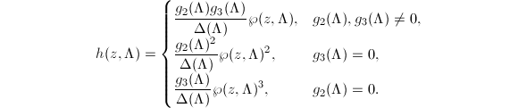
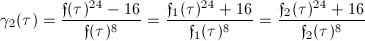
Now let us introduce Weber's method for computing the singular moduli of integer values. The main tool of Weber's computation is a class of Weber functions  ,
,  ,
,  and
and  (not to be confused with the Weber function defined earlier).
Definition 6
Define the Weber function ![$$\gamma_2(\tau)=\sqrt[{3}]{j(\tau)}=12\frac{g_2(\tau)}{\sqrt[{3}]{\Delta(\tau)}}, $$](./latex/latex2png-MinorThesis3_127498776_.gif) where
where ![$\sqrt[{3}]{\Delta(\tau)}$](./latex/latex2png-MinorThesis3_34206865_-6.gif) is chosen so that it is real-valued on the imaginary axis.
is chosen so that it is real-valued on the imaginary axis.
where is chosen so that it is real-valued on the imaginary axis.
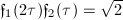
The Weber function satisfies the following transformation property  Then it is straightforward to check that
  is a modular function with respect to
  ([3, 12.3]). So
  . Moreover, when the order
  has discriminant prime to 3, we have the following even better relationship between and ([3, 12.2]).
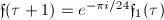
Theorem 11
Let be an order of discriminant  and assume
  . Set
. Set 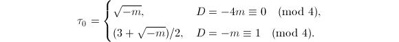 Then
Then  .
.  is an algebraic integer and
  is the ring class field of . Moreover,
  .
.
be an order of discriminant and assume . Set
Then . is an algebraic integer and is the ring class field of . Moreover, .
By the last part of Theorem 11, we know that has the same degree as  when . In particular, when , is an integer since is so. Therefore
 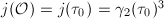 is a cube when , which coincides with the result listed in Table 1 . The two boxed exceptions
 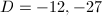 , as expected, are divisible by 3.
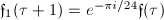
 be the Dedekind
  -function. We define the Weber functions
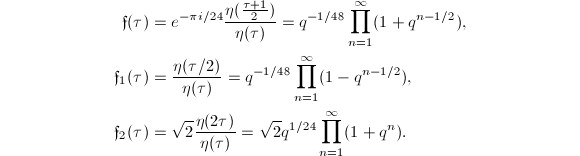
We may summarize the most important relationship and transformation properties of these Weber functions as follows [3, 12.17, 12.19]. These properties are crucial to Weber's computation of singular moduli.
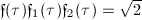 .
. .
. .
. ,
,  ,
,  .
. ,
,  ,
, Now let us use Theorem 12 to compute for those orders with discriminants prime to 3. As a consequence, we will be able to compute the singular moduli for those orders easily by raising the corresponding to the third power.
 . Then for
  ,
,  and for
  ,
,  where
where  is the nearest integer function.
Proof
First consider the case of even discriminant. By Theorem 12 (c), we know that
 Using the product formula, we get
  Now applying the inequality
  for
for  , we obtain
  since
since  . Using this estimate and plugging
  into Equation (1), we get
  The difference of the upper bound and the lower bound is
  Using the inequality
  for
for  , we have
  The right hand side is an increasing function in , so
  implies
  . But is an integer by Theorem 11, so
  .
.
Using the product formula, we get Now applying the inequality for , we obtain since . Using this estimate and plugging into Equation (1), we get The difference of the upper bound and the lower bound is Using the inequality for , we have The right hand side is an increasing function in , so implies . But is an integer by Theorem 11, so .
Next let us consider the case of odd discriminant. The above computation fails, since  is now negative. However, we can translate
  to
to  as follows. By Theorem 12 (b) and (d), we know that
  and
and  Therefore
  Now a similar argument shows the desired result
  .
□
.
□
Example 4
Consider  . Then
  , so by Theorem 11 and Theorem 13, we can compute the singular modulus
 It agrees with the result in Table 1 . We will come back to this example using the powerful Gross-Zagier's theorem in the next section.
. Then , so by Theorem 11 and Theorem 13, we can compute the singular modulus
It agrees with the result in Table 1 . We will come back to this example using the powerful Gross-Zagier's theorem in the next section.
Gross-Zagier's theorem on singular moduli
Gross and Zagier [8] proved a result which completely determines the prime factorization of the norm of the difference between two singular moduli, which in turn justified many classical conjectures on the congruences of singular moduli proposed by Berwick [9]. They provide two proofs of different natures: The first proof, an algebraic proof, is based on Deuring's work on endomorphism rings of elliptic curves mentioned in Chapter 2. The second analytic proof relies on the calculation of the Fourier coefficients of the restriction to the diagonal  of an Eisenstein series of the Hilbert modular group of
  . As the authors remarked, these two methods can be viewed as the special case
  of the theory of local heights of Heegner points on , which generalizes to the groundbreaking Gross-Zagier formula [10].
In this section, we will first state Gross-Zagier's theorem, then use it to compute several examples and derive some consequences. At the end, we will discuss a bit of the algebraic proof of Gross-Zagier's theorem.
Now consider two orders with discriminants  and
and  satisfying
  . Let
. Let  be the numbers of their units and
  be their class numbers. Let
  and
and  be the representatives of their ideal class groups. Define
  Notice that when
  (e.g.,
  ),
),  is just the norm of any of the differences
  . In general, is a certain power of this norm and
  is always an integer.
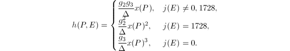
To state Gross-Zagier's theorem, let us introduce some notation. Let  . For a prime , define
  This is well-defined whenever
  . More generally, if has the prime factorization
  with
with  , we define
  Finally, set
  This is well-defined whenever all primes dividing satisfy . Now the main theorem is as follows.
Example 5
When  , we know the corresponding
  and
and  . So in this case,
  In particular, for
  ,
,  and
and  , so we have
  . The factors of
  are tabulated in Table 2 , so we can conclude (after figuring out the sign) that
  which agrees with our computation in Example 4.
, we know the corresponding and . So in this case, In particular, for , and , so we have . The factors of are tabulated in Table 2 , so we can conclude (after figuring out the sign) that which agrees with our computation in Example 4.
Example 6
Similarly, when  , we know the corresponding
  and
and  . So in this case,
  In particular, for , we have
  . The factors of
  are tabulated in Table 3 , so we can conclude (after figuring out the sign) that
  which also agrees with our computation in Example 4.
, we know the corresponding and . So in this case, In particular, for , we have . The factors of are tabulated in Table 3 , so we can conclude (after figuring out the sign) that which also agrees with our computation in Example 4.
As we have noticed, the prime factor of  is always a factor of
  . In fact, we have the following interesting result concerning the function ([3, Exercise 13.15, 13.16]).
 where
where  and
and  . In this case,
Corollary 1
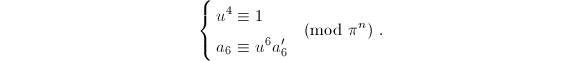
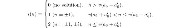
Let be a prime dividing , then divides a positive integer of the form . In particular,  . Moreover,
  and .
and .
be a prime dividing , then divides a positive integer of the form . In particular, . Moreover, and .
Proof
The first part follows immediately from Lemma 4. For the second part, by Lemma 4, we have  for such . Without loss of generality, we may assume
  . But since
  for some , therefore
  .
□
.
□
for such . Without loss of generality, we may assume . But since for some , therefore .
□
Now we can explain the phenomenon we observed in Table 1 . Suppose is a prime dividing an integer singular modulus of discriminant , or equivalently, dividing  , then by Corollary 1, we have
  . So these singular moduli have relatively small prime factors, though their own values can be fairly huge.
Finally, let us come to the algebraic proof of Gross-Zagier's theorem. The proof proceeds locally. As the first step, Gross and Zagier relate the valuation of the difference of two -values to the geometry of elliptic curves and reduce it to a counting problem of isomorphisms between elliptic curves. Next, a generalization of Deuring's lifting theorem will allow one to reduce the problem to counting certain subrings of the endomorphism ring of a supersingular elliptic curve. To complete the proof, Gross and Zagier give a convenient description of a maximal order and its subrings in the rational quaternion algebra ramified at  and a prime for explicit computation.
The first step can be viewed as an interesting geometrical interpretation of the difference of -values.
Theorem 15
Let  be a complete discrete valuation ring whose quotient field has characteristic zero and whose residue field is algebraically closed and has characteristic
  (e.g.,
  ). Let
  be its uniformizer and be its normalized valuation. Let
  be elliptic curves defined over with good reduction and -invariants
  . Denote the set of isomorphisms from to
  defined over
  by
by  . Then
be a complete discrete valuation ring whose quotient field has characteristic zero and whose residue field is algebraically closed and has characteristic (e.g., ). Let be its uniformizer and be its normalized valuation. Let be elliptic curves defined over with good reduction and -invariants . Denote the set of isomorphisms from to defined over by . Then
Proof We may assume that are isomorphic over the algebraically closed field  , otherwise both sides are zero. Denote
  , then
  .
.
are isomorphic over the algebraically closed field , otherwise both sides are zero. Denote , then .
Let us consider the case when  for simplicity. Change models for with simplified Weierstrass equations
By definition, we have  if and only if we can solve the congruences
 simultaneously for some unit
  . In this case
  , and at least one of
  and
and  is a unit in
  since has good reduction mod .
If is a unit in , then  is also a unit. By changing models we may assume that
  . Then
  On the other hand, the congruences become
 We may possibly modify
  by
by  so that
  is maximal. Then
 We get
  So the theorem holds in this case.
If is a unit in , then  is also a unit. Similarly by changing models we may assume that
  . Then
 where
where  is a primitive cube root of unity in . On the other hand, the congruences become
 We may possibly modify
  by or
by or  so that
  is maximal. Then
 We get
  This completes the proof.
□
This completes the proof.
□
For simplicity, we will assume  is a prime from now on (for the general case, see [11]). Let be the ring of integers of
  . Let be an elliptic curve over with complex multiplication by and with -invariant
  . For our purpose, we need to calculate
  where is an elliptic curve over with complex multiplication by some ring
 ![$\mathbb{Z}[w]$](./latex/latex2png-MinorThesis3_28092862_-5.gif) of discriminant . We can rewrite in a manner which only depends on . Suppose
of discriminant . We can rewrite in a manner which only depends on . Suppose  , then
  is an endomorphism of mod
  , which has the same norm, trace and action on tangent space as
  . Namely,
  belongs to the set
  Conversely, every element of
  is of the form for some unique ensured by the following lifting theorem, which is a refinement of Deuring's lifting theorem ([12, 14.14]).
Theorem 16
Let  be an elliptic curve over and
  . Assume that
 ![$\mathbb{Z}[\alpha_0]$](./latex/latex2png-MinorThesis3_162559240_-5.gif) is a -module of rank 2 and is integrally closed in its quotient field. Suppose
is a -module of rank 2 and is integrally closed in its quotient field. Suppose  induces multiplication by a quadratic element
  on
on  . If there exists
  such that
  then there exists an elliptic curve over and
  , such that
  reduces to
  mod and induces multiplication by on
  . Moreover, if
  is another lifting, then there is a commutative diagram
 ![$$\xymatrix{E \ar[r]^\alpha\ar[d]_{\cong} & E \ar[d]^{\cong}\\ E'\ar[r]^{\alpha'} & E'.}$$](./latex/latex2png-MinorThesis3_69540335_.gif)
be an elliptic curve over and . Assume that is a -module of rank 2 and is integrally closed in its quotient field. Suppose induces multiplication by a quadratic element on . If there exists such that then there exists an elliptic curve over and , such that reduces to mod and induces multiplication by on . Moreover, if is another lifting, then there is a commutative diagram
Now by Theorem 16, we reduce to the counting problem of .
When  ,
,  splits in
  , so has ordinary reduction mod and
  ([12, 13.12]). But contains no elements of discriminant , so is empty for all
  . (Another way to say this: if two elliptic curves and with complex multiplication have the isomorphic reduction
  , then the reduction must be supersingular, since two different orders and
  have to embed into
  simultaneously.)
So we only need to consider the case  and has supersingular reduction. Then
  is a maximal order in the rational quaternion algebra ramified at and by Theorem 8. The algebra can be desribed explicitly as a subring of
  ,
,  The subrings
  can also be desribed explicitly. Using these descriptions, it turns out that in many cases
  equals to
  times the number of the solutions
  (under certain conditions on ) of the equation
  where we assume
  is a prime . The more precise result is the following.
 where
where  and
and  is the number of ideals of
 The main Theorem 14 now can be derived directly from Equation 2using the formula  Unfortunately, we will omit the details here.
References
[1]Introduction to the Arithmetic Theory of Automorphic Functions, Princeton University Press, 1971.
[2]Complex multimplication, Algebraic Number Theory, London Mathematical Society, 1967, 292-296.
[3]Primes of the Form $X^2 + ny^2$: Fermat, Class Field Theory, and Complex Multiplication, John Wiley \& Sons, 1989.
[4]Algebraic Number Theory, Springer, 1994.
[5]Complex multimplication and explicit class field theory, 1996, Senior thesis, Harvard University.
[6]Advanced Topics in the Arithmetic of Elliptic Curves, Springer, 1994.
[7]A First Course in Modular Forms, Springer, 2010.
[8]On singular moduli, J. reine angew. Math 355 (1985), no.2, 191--220.
[9]Modular Invariants Expressible in Terms of Quadratic and Cubic Irrationalities, Proc. London Math. Soc. 28 (1927), 53-69.
[10]Heegner points and derivatives of L-series, Invent. math 84 (1986), no.2, 225--320.
[11]Prime factorization of singular moduli, Brown University, 1984.
[12]Elliptic Functions, Springer, 1987.