- Motivation
- Weil cohomology
- Algebraic de Rham cohomology
- De Rham cycle class maps (via Chern characters)
- Formalism of cohomological correspondences
- Formal consequences of a Weil cohomology
- Intersecting cycles
- Adequate equivalences on algebraic cycles
- Tannakian theory
- The Kunneth Standard Conjecture (Conjecture C)
- The Lefschetz Standard Conjecture (Conjecture B)
- The Hodge Standard Conjecture (Conjecture I)
- Absolute Hodge cycles
- Motivated cycles
- The Motivated variational Hodge conjecture
- Mumford-Tate groups
- Applications of the motivated variational Hodge conjecture
- Rigid local systems
- Perverse sheaves
- The middle convolution
- Katz's classification
-
Local systems of type

- Universal rigid local systems
- Middle convolution with parameters
These are my live-TeXed notes for the course Math 268x: Pure Motives and Rigid Local Systems taught by Stefan Patrikis at Harvard, Spring 2014.
Any mistakes are the fault of the notetaker. Let me know if you notice any mistakes or have any comments!
[-] Contents
01/28/2014
 Motivation
Let  be a field with algebraic closure
  (so
(so  ). Consider smooth projective varieties
  over (either dropping the word smooth or projective will force us to enter the world of mixed, rather than pure, motives). There are several nice cohomology theory.
- the Betti realization
 (a
(a  -vector space), the singular cohomology of the topological space
  .
. - the de Rham realization
 (a -vector space with a Hodge filtration), the algebraic de Rham cohomology = the hypercohomology of the sheaf
  of algebraic differential forms on .
 - the
 -adic realization
  (a
(a  -vector space with
  -action), the -adic etale cohomology.
It is not even clear a priori that these -vector space, -vector space and -vector have the same dimension. But miraculously there are comparison isomorphisms between them. For example,

These isomorphisms are functorial and satisfy other nice properties (indeed an isomorphism of Weil cohomology, more on this later). This suggests that there is an underlying abelian category (of pure motives) that provides the comparison between different cohomology theory.
Slogan "sufficient geometric" pieces of cohomology have comparable meaning in all cohomology theory
We will spend a great amount of time on the foundation of all these different cohomology theory. But notice the comparison isomorphisms already suggest the various standard conjectures, for examples,
- Standard conjecture D: numerical equivalence = cohomological equivalence
- Standard conjecture C: Kunneth (the category of pure motives is graded and has a theory of weights).
- Standard conjecture B: Lefschetz (the primitive cohomology should be "sufficiently geometric")
Question
Why should one care about the existence of such a category?
One motivation is that one gets powerful heuristic for transferring the intuition between different cohomology theory.
Example 1
By the early 60's, one knew that if  is a smooth projective variety, then it follows from Hodge theory that
  naturally carries a pure Hodge structure of weight , i.e. a -vector space
  with a bi-grading
  such that
  , where
  is the complex conjugation with respect to
  . On the other hand, Weil had conjectured that for a smooth projective variety
  . The
. The  -representation
  is pure of weight , in the sense that the eigenvalues
  of the geometric Frobenius
  are algebraic numbers and for each embedding
  of into the complex numbers,
  .
.
is a smooth projective variety, then it follows from Hodge theory that naturally carries a pure Hodge structure of weight , i.e. a -vector space with a bi-grading such that , where is the complex conjugation with respect to . On the other hand, Weil had conjectured that for a smooth projective variety . The -representation is pure of weight , in the sense that the eigenvalues of the geometric Frobenius are algebraic numbers and for each embedding of into the complex numbers, .
When is smooth but not projective, people played with examples and found that can be filtered (the weight filtration) such that the Frobenius eigenvalue is pure on each graded piece.
Example 2
Let be a smooth projective curve,  be a finite set of points and
  . Then we have an exact sequence
  Here
Here  is pure of weight 1 and
  (
( , the -adic cyclotomic character) is pure of weight 2 and
  is also pure of weight 2. Therefore one obtains an increasing weight filtration on
  :
: 
be a smooth projective curve, be a finite set of points and . Then we have an exact sequence Here is pure of weight 1 and (, the -adic cyclotomic character) is pure of weight 2 and is also pure of weight 2. Therefore one obtains an increasing weight filtration on :
The above mentioned -adic intuition (generalized to higher dimension) lead Deligne to mixed Hodge theory. To give  a mixed Hodge structure for not smooth projective, the key point is to find a spectral sequence
  such that its
  term is (conjecturally) pure of weight
  .
.
In Hodge II, Deligne treated the case of smooth but no longer projective varieties  . The (-adic analogue of the) spectral sequence is the Leary spectral sequence for
  , where a smooth compactification of
  with
with  is a union of smooth divisors with normal crossings,
  One can explicitly compute the sheaf
  where
where  is smooth. Therefore
  is pure of weight .
Let us look at the differential  : notice both the target and the source are pure of weight (all
  are pure of weight ), nothing is weired. But on the
  -page,
  , where the source has weight and the target has weight
  respectively. The mismatching of the weight of the Frobenius eigenvalues implies that
  for
for  . Therefore the Leray spectral sequence degenerates at -page. One can compute that
  The Betti analogue (of maps of pure Hodge structure) is provided by the reinterpretation that
  and the differentials
  's are simply Gysin maps ( = Poincare dual to pullbacks), which are also maps of pure Hodge structures.
The upshot is that the -adic Leray spectral sequence gives the weight filtration (= the Leary filtration up to shift), and the graded piece  is pure of weight
  . The Betti Leray sequence also gives a weight (defined to be) filtration on
  such that we already know that
  are naturally pure Hodge structures.
Another motivation for considering the category of pure motives is toward a motivic Galois formalism.
Example 3
Let be a field. The classical Galois theory establishes an equivalence between finite etale -schemes with finite sets with  -actions. Linearizing a finite set
  with
with  -action gives finite dimensional -vector spaces
  with the continuous -action
  . The linearization of finite etale -schemes are the Artin motives (motives built out of zero dimension motives). The equivalence between the two linearized categories is then given by
  .
.
be a field. The classical Galois theory establishes an equivalence between finite etale -schemes with finite sets with -actions. Linearizing a finite set with -action gives finite dimensional -vector spaces with the continuous -action . The linearization of finite etale -schemes are the Artin motives (motives built out of zero dimension motives). The equivalence between the two linearized categories is then given by .
Generalizing to higher dimension: the category of finite etale -schemes is extended to the category of pure homological motives. The Standard conjectures then predict that it is equivalent to the category of representations of a certain group  , which is a extension of classical Galois theory
  These are still conjectural. But one can replace the category of pure homological motives by something closely related and obtain unconditional results. In this course we will talk about one application of Katz's theory of rigid local systems (these are topological gadgets but surprisingly produce motivic examples): to construct the exceptional as a quotient of
  (the recent work of Dettweiler-Reiter and Yun).
01/30/2014
Weil cohomology
We now formulate the notion of Weil cohomology, in the frame work of motives.
Definition 1
Let  be a field. Let
  be smooth projective (not assumed to be connected) variety over . Let
  be the category of such varieties. Then is a symmetric monoidal via the fiber product
  with the obvious associative and commutative constraints and the unit
  .
.
be a field. Let be smooth projective (not assumed to be connected) variety over . Let be the category of such varieties. Then is a symmetric monoidal via the fiber product with the obvious associative and commutative constraints and the unit .
Definition 2
Let  be a field. Let
  be the category of finite dimensional graded -vector spaces in degrees
  with the usual tensor operation
  It is endowed with a graded commutative constraint via
be a field. Let be the category of finite dimensional graded -vector spaces in degrees with the usual tensor operation It is endowed with a graded commutative constraint via
Definition 3
A Weil cohomology over (a field of characteristic 0) on is a tensor functor  , namely,
  comes with a functorial (Kunneth) isomorphisms
  respecting the symmetric monoidal structure. Notice the monoidal structure induces a cup product
  making
  a graded commutative -algebra. We require it to satisfy the following axioms.
(a field of characteristic 0) on is a tensor functor , namely, comes with a functorial (Kunneth) isomorphisms respecting the symmetric monoidal structure. Notice the monoidal structure induces a cup product making a graded commutative -algebra. We require it to satisfy the following axioms.
- (normalization)
 . In particular,
  is invertible in
  . We define the Tate twists
  (this is well motivated by -adic cohomology).
 - (trace axiom) For any of (equi-)dimension
 , there is a trace map
  satisfying
- Under
 , one has
  .
.  and the cup product induces a perfect duality (Poincare duality)
- Under
- (cycle class maps) Let
 be the -vector spaces with a basis consisting of integral closed schemes
  of codimension
  . Then there are cycle class maps
  satisfying
 factors through the Chow group
  (modulo the rational equivalence).
- is contravariant in , i.e., for a morphism
 and a cycle of codimension , we have
 ![$$f^*\gamma_Y^r(Z)=\gamma_X^r([f^{-1}Z])$$](./latex/latex2png-PureMotives_140904715_.gif) whenever this makes sense. This will always make sense after passing to the Chow group. In general, one cannot always define
whenever this makes sense. This will always make sense after passing to the Chow group. In general, one cannot always define  on
on  . But if
  is flat , then one can: in fact, by flatness has all its components of codimension in (but is not necessarily integral). Let
  be the (reduced structure) of the irreducible components. One then associates a cycle
 ![$$[f^{-1}Z]:=\sum n_i W_i,$$](./latex/latex2png-PureMotives_53293601_.gif) where
where  , the length of the local ring at . We also require it to be compatible with pushforward (defined in Definition 10) that
- For
 ,
,  .
.  Notice
  is not necessarily a combination of integral closed subscheme (e.g.,
 ![$\mathbb{F}_p(\sqrt[p]{t}) \otimes_{\mathbb{F}_p} \mathbb{F}_p(t)\cong\mathbb{F}_p[X]/X^p$](./latex/latex2png-PureMotives_102787841_-6.gif) is nonreduced), the cycle should be understood as the reduced structure with multiplicity.
is nonreduced), the cycle should be understood as the reduced structure with multiplicity. - (pinning down the trace) the composite
 sends
sends  to
to ![$\sum n_i [k(P_i):k]$](./latex/latex2png-PureMotives_92716811_-5.gif) , where
, where  are closed points.
Remark 1
Sometimes the Lefschetz axiom is also thrown in the definition of Weil cohomology. We will talk about this later.
Remark 2
We set  . This means via the comparison isomorphism,
  the image of
  is
is  . If we take granted that the comparison isomorphisms are compatible with Mayer-Vietoris. Applying Mayer-Vietoris to
  , then we are reduced to the calculation on
  (
( ). The isomorphism
  is given by
  here
here  is a smooth 1-chain. A good -basis of
  is given by the differential
  . Choosing a simple loop around the origin, then one obtains
  .
.
. This means via the comparison isomorphism, the image of is . If we take granted that the comparison isomorphisms are compatible with Mayer-Vietoris. Applying Mayer-Vietoris to , then we are reduced to the calculation on (). The isomorphism is given by here is a smooth 1-chain. A good -basis of is given by the differential . Choosing a simple loop around the origin, then one obtains .
Example 4 (Trace in Betti cohomology)
Let be smooth projective of dimension . Define to be the composite ![$$\scriptstyle H^{2d}_B(X)(d)\xrightarrow{\frac{1}{(2\pi i)^d}} H^{2d}_B(X)\xrightarrow[\alpha]{\sim} H^{2d}(X, \underline{\mathbb{Q}})\rightarrow H^{2d}(X,\underline{\mathbb{Q}}) \otimes \mathbb{R} \xrightarrow[\beta]{\sim} H^{2d}(X,\mathcal{A}_X^\cdot)\xrightarrow{\int_X}\mathbb{R},$$](./latex/latex2png-PureMotives_229627239_.gif) where
where  is the smooth de Rham complex with
  -coefficients. Notice is an isomorphism because the sheafy singular cochain complex is a flasque resolution of
  and
and  is an isomorphism because is a fine resolution of
  . The choice
  will chancel out the choice of the orientation we made on complex manifold when we do integration and one can check that
  lands in .
be smooth projective of dimension . Define to be the composite where is the smooth de Rham complex with -coefficients. Notice is an isomorphism because the sheafy singular cochain complex is a flasque resolution of and is an isomorphism because is a fine resolution of . The choice will chancel out the choice of the orientation we made on complex manifold when we do integration and one can check that lands in .
Algebraic de Rham cohomology
Suppose is a field of characteristic 0 and smooth (not necessarily projective).
Definition 4
We define the algebraic de Rham cohomology  to be the hypercohomology of the sheaf of algebraic differential forms on .
to be the hypercohomology of the sheaf of algebraic differential forms on .
 is a Weil cohomology.
We now selectively check a few of the axioms.
Proof
Given a morphism  . Let
. Let  be an injective resolution of
  and
and  be an injective resolution of
  . Then
  is quasi-isomorphic to
  . The map
  induces the pull-back on

. Let be an injective resolution of and be an injective resolution of . Then is quasi-isomorphic to . The map induces the pull-back on
The Kunneth isomorphism is explicitly given by  , where
  and
and  are the natural projections.
□
are the natural projections.
□
Remark 3
To check that  is finite dimensional for smooth projective, one can use the Hodge to de Rham spectral sequence
  and the fact that each
  is finite dimensional (this may fail when is not projective) and
  lives in a bounded region. For not necessarily projective or smooth varieties, is still finite dimensional (by comparison, and by the resolution of singularities in characteristic 0). may fail to be finite dimensional in characteristic
  for nonprojective varieties (see the next example).
is finite dimensional for smooth projective, one can use the Hodge to de Rham spectral sequence and the fact that each is finite dimensional (this may fail when is not projective) and lives in a bounded region. For not necessarily projective or smooth varieties, is still finite dimensional (by comparison, and by the resolution of singularities in characteristic 0). may fail to be finite dimensional in characteristic for nonprojective varieties (see the next example).
Example 5
When is affine, we have  (this follows from the vanishing of
  for affine and
  quasi-coherent; in particular, ), which makes the computation feasible. For example, the de Rham complex for
  is simply
 ![$k[T]\xrightarrow{d}k[T]dT$](./latex/latex2png-PureMotives_29759566_-5.gif) . So taking cohomology gives
. So taking cohomology gives  and
and  . This also gives an example in characteristic that
  is infinite dimensional because
  , so one don't really want to work with the algebraic de Rham cohomology in characteristic !
is affine, we have (this follows from the vanishing of for affine and quasi-coherent; in particular, ), which makes the computation feasible. For example, the de Rham complex for is simply . So taking cohomology gives and . This also gives an example in characteristic that is infinite dimensional because , so one don't really want to work with the algebraic de Rham cohomology in characteristic !
02/04/2014
In general, one covers by open affines  . For any quasi-coherent sheaf on , one then obtains the Cech complex
  , a resolution of by acyclic sheaves, defined by
  Now we have a double complex
 ![$$\xymatrix{\mathcal{C}^\cdot(\mathcal{U},\mathcal{O}_X) \ar[r] & \mathcal{C}^\cdot(\mathcal{U},\Omega_X^1) \ar[r] & \mathcal{C}^\cdot(\mathcal{U},\Omega_X^2) \ar[r] &\cdots\\ \mathcal{O}_X \ar[r] \ar[u]^{\sim} & \Omega_X^1 \ar[r] \ar[u]^{\sim}& \Omega_X^2 \ar[r] \ar[u]^{\sim}& \cdots}$$](./latex/latex2png-PureMotives_88628631_.gif) whose columns are acyclic resolutions of
whose columns are acyclic resolutions of  . The general formalism implies that
  the cohomology of the global sections of the total complex. Recall the total complex is defined by
  where
where  .
.
Example 6 (normalization)
Let  and
and  be a covering of
  . The Cech double complex looks like
 ![$$\xymatrix{ \mathcal{O}(U_0\cap U_1)\ar[r] & \Omega^1(U_0\cap U_1)\\ \mathcal{O}(U_0)\oplus\mathcal{O}(U_1) \ar[r] \ar[u] & \Omega^1(U_0)\oplus\Omega^1(U_1) \ar[u]}$$](./latex/latex2png-PureMotives_28170513_.gif) The total complex is thus
The total complex is thus  where the two differentials are given by
  and
and  One can easily compute
  ,
,  and
and  is 1-dimensional generated by
  . Indeed one sees the computation really shows
  This is an instance of the Hodge to de Rham spectral sequence.
and be a covering of . The Cech double complex looks like The total complex is thus where the two differentials are given by and One can easily compute , and is 1-dimensional generated by . Indeed one sees the computation really shows This is an instance of the Hodge to de Rham spectral sequence.
Remark 4
The Hodge de Rham spectral sequence comes from filtering the total complex of the double complex  . Take the filtration (cut out by right half planes)
  So
So  itself forms a complex. The general machinery implies that the spectral sequence associated to this filtered complex is
  Here
Here  defines the filtration on
  (so the grading on the right hand side makes sense). Notice in our case,
  is simply
  and
and  is nothing but .
. Take the filtration (cut out by right half planes) So itself forms a complex. The general machinery implies that the spectral sequence associated to this filtered complex is Here defines the filtration on (so the grading on the right hand side makes sense). Notice in our case, is simply and is nothing but .
Remark 5
What happens when one filter the total complex in the other way (by upper half planes)? Namely  Then we see that
  . The corresponding sequence is the Mayer-Vietoris spectral sequence. When the covering
  consists of two affines, it recovers the usual Mayer-Vietoris long exact sequence.
Then we see that . The corresponding sequence is the Mayer-Vietoris spectral sequence. When the covering consists of two affines, it recovers the usual Mayer-Vietoris long exact sequence.
Theorem 3
If and is projective, then the Hodge to de Rham spectral sequence degenerates at the  -page.
and is projective, then the Hodge to de Rham spectral sequence degenerates at the -page.
To define the trace for the algebraic de Rham cohomology, we proceed in two steps. We first show that  is abstractly the right thing, i.e.,
  and is if is geometrically connected. Then we pin down that actual map
  after defining the de Rham cycle class map.
The first step uses the Serre duality. By the Hodge to de Rham spectral sequence, we have a map  By Serre duality (
 is the dualizing sheaf), one has the trace map
  So we want to say that the map
  is an isomorphism. By the Hodge de Rham spectral sequence, it is enough to show that
  (or
(or  because
  is a free
  -module of rank 1). This can be checked bare-handed by reduction to
  : choose a finite flat map
  to get the trace map
  (so
(so  ). It follows that
  is injective. It suffices to prove that
  which boils down to the direct computation that
  using the Hodge to de Rham spectral sequence.
To pin down , we need to choose carefully a generator  of
of  and set
 ![$$\tr_X(c\cdot u_X)=\frac{\tr_{H^0(X,\mathcal{O}_X)/k}(c)}{[H^0(X,\mathcal{O}_X):k]},$$](./latex/latex2png-PureMotives_144211552_.gif) i.e.,
i.e.,  .
.
De Rham cycle class maps (via Chern characters)
We seek a cycle class map such that ![$\tr_X\gamma_X^d(P)=[k(P):k]$](./latex/latex2png-PureMotives_66976247_-5.gif) as follows.
as follows.
- Define the Chern class
 of line bundles.
 - Define the Chern class
 of vector bundles.
 - Define the Chern character
 of vector bundles on .
 - One knows that
 factors through
  , Grothendieck group of vector bundles on . Using the fact that is smooth, the latter can be identified with
  , the Grothendieck group of coherent sheaves on .
 - For a codimension cycle,
 makes sense and we define the cycle class map
Now we describe each step in details.
Step a
We want a group homomorphism  . Identify
  . The map
  induces a map
 ![$\mathcal{O}_X^\times\rightarrow \Omega_X^\cdot[1 ]$](./latex/latex2png-PureMotives_250186528_-5.gif) and hence induces the desired map
and hence induces the desired map  .
.
Step b
Let be a vector bundle of rank on . Denote the projective bundle  . Notice
  on
on  has a tautological line subbundle
  . Let
. Let  . The fact (the Leray-Hirsch theorem, a special case of the Leray spectral sequence) is that
  is a free module over
  with basis
  . We then define
  by
by  Notice this agrees with the previous definition of of line bundles and is functorial in .
02/06/2014
Define the total Chern class  The key is the following multiplicative property.
 we have
  .
.
Proof
To show this, one first show that if  is a direct sum of line bundles, then
  Then reduce the general to the first case by showing that there exists a map
  such that
  splits as direct sum of line bundles and
  is injective on (the splitting principle).
is a direct sum of line bundles, then Then reduce the general to the first case by showing that there exists a map such that splits as direct sum of line bundles and is injective on (the splitting principle).
For the first case, since the statement is invariant under twist, one can assume each  is very ample of the form
  and reduce to the case to the case of being a product of projective spaces. Notice that each gives a section
  and by definition
  . Write
  . Pullback the defining relation for
  along each
  , we obtain the relation
  So the polynomial
  in
in ![$H^*(X)[t]$](./latex/latex2png-PureMotives_223510292_-5.gif) has roots
has roots  . But has the advantage of being like a polynomial ring,
 ![$$H^*\left(\prod_{i=1}^r \mathbb{P}^{d_i}\right)\cong k[x_1,\ldots,x_r]/(x_1^{d_i+1},\ldots, x_r^{d_r+1}).$$](./latex/latex2png-PureMotives_80461833_.gif) Assume
Assume  , then the defining relation must be
  , which shows that is the
  -th symmetric polynomial of
  as desired.
To reduce the general case to the first case, arrange  so that
  has a full flag of subbundles by iterating the projective bundle construction, then split the extension by further pullback: if one has a surjection
  of vector bundles, then the sections
  form an affine bundle over ; pulling back along this affine bundle splits and induces an isomorphism on cohomology.
□
form an affine bundle over ; pulling back along this affine bundle splits and induces an isomorphism on cohomology.
□
Step c
Using the multiplicative property, we can define formally the Chern roots of so that  . Here the Chern roots don't not make sense but their the symmetric polynomials do make sense in cohomology. Define the Chern character
  This makes sense in cohomology. Now we have the additivity
  in exact sequences. Moreover
  . Therefore we obtain a ring homomorphism
When is smooth, one can form finite locally free resolutions of any coherent sheaves on , and taking the alternating sum of the terms in the resolutions induces the inverse of natural map  . Thus
  (see Hartshorne, Ex III.6.8).
Step d
For a codimension cycle, makes sense and we define the cycle class map  In particular, our choice of the basis for
  is given by for any closed point
  of ,
of , ![$$u_X=\frac{\gamma_X^d(P)}{[k(P):k]}=\frac{\ch_d(k(P))}{[k(P):k]}.$$](./latex/latex2png-PureMotives_190714729_.gif) This is the choice we made to normalize the trace map. We need to check that is independent on the choice of (this follows from connecting two points by a curve in and the invariance of
This is the choice we made to normalize the trace map. We need to check that is independent on the choice of (this follows from connecting two points by a curve in and the invariance of  in a flat family). We also need to check that
  . This reduce to the case of projective spaces. Let
  be a closed point. One can put in a chain
  Using the short exact sequences of the form (given a choice of a section of
  ),
),  for each , it follows that in , we have
  Applying the Chern character we obtain that for
  ,
,  which is nonzero.
Formalism of cohomological correspondences
Let  be a Weil cohomology.
Definition 5
Given a morphism , we define the Gysin map  to be the transpose of under the Poincare duality. At the level of cycles,
  is basically
  when
when  and zero otherwise (this matches the degree shift in
  ).
).
, we define the Gysin map to be the transpose of under the Poincare duality. At the level of cycles, is basically when and zero otherwise (this matches the degree shift in ).
 ,
,  , then
  .
.
Proof
The property  characterizes .
□
characterizes .
□
characterizes .
□
Remark 7
Using Gysin maps, one has an alternative construction of cycle class maps. For a smooth cycle  of codimension , we define
 ![$$\gamma_X^p(Z)=i_*[Z],$$](./latex/latex2png-PureMotives_162947520_.gif) where
where ![$[Z]$](./latex/latex2png-PureMotives_16741396_-5.gif) is "1" in
is "1" in  . This can be extended to non-smooth cycles by a resolution
  and defining
 ![$\gamma_X^p(Z)=\tau_*[\tilde Z]$](./latex/latex2png-PureMotives_208863650_-5.gif) .
.
of codimension , we define where is "1" in . This can be extended to non-smooth cycles by a resolution and defining .
Definition 6
A cohomological correspondence from to  is an element
  interpreted (using the Poincare duality and the Kunneth formula) as a linear map
  . Explicitly, if
  , then
  (extended to be zero away from top degree). Let
  ,
,  be the natural projections. Then another way of writing
  is
is  Namely, pullback
  , intersect with
  , then pushforward to . One can check that
  by the projection formula.
to is an element interpreted (using the Poincare duality and the Kunneth formula) as a linear map . Explicitly, if , then (extended to be zero away from top degree). Let , be the natural projections. Then another way of writing is Namely, pullback , intersect with , then pushforward to . One can check that by the projection formula.
 ,
,  .
.
 of
of  under
under  . One can check that
  .
.
 , we define
  .
.
 .
.
Proof
Notice that  . The claim then follows from the associativity of composition of correspondences. For details, see Fulton, Intersection theory, Chapter 16.
□
. The claim then follows from the associativity of composition of correspondences. For details, see Fulton, Intersection theory, Chapter 16.
□
. The claim then follows from the associativity of composition of correspondences. For details, see Fulton, Intersection theory, Chapter 16.
□
 be the graph of the morphism
  ,
,  ,
,  .
.
Our next goal is to deduce the Weil conjecture (except the Riemann hypothesis) from a Weil cohomology (hence the name). We will later see that the Riemann hypothesis follows from the standard conjectures.
02/11/2014
Formal consequences of a Weil cohomology
Let be a Weil cohomology.
Proposition 3 (Lefschetz fixed point)
Suppose is algebraically closed. Let  be connected. If
  ,
,  are of degree
  and
and  respectively (namely,
  and induces
  ; similar for
  ). Then
is algebraically closed. Let be connected. If , are of degree and respectively (namely, and induces ; similar for ). Then
Proof
We compute by each Kunneth component so let  ,
,  . Let
. Let  be a basis of
  and let
  be a dual basis of
  such that
  . So we can write
  Here
Here  So the left hand side is equal to
 Switching
  and
and  introduces another sign
  which cancels out the sign
  since
since  . So the left hand side is equal to
  To compute the trace on the right hand side, we notice that
  Since we care only about the
  -term when taking the trace, this matches the left hand side.
□
-term when taking the trace, this matches the left hand side.
□
, . Let be a basis of and let be a dual basis of such that . So we can write Here So the left hand side is equal to
Switching and introduces another sign which cancels out the sign since . So the left hand side is equal to To compute the trace on the right hand side, we notice that Since we care only about the -term when taking the trace, this matches the left hand side.
□
Let  be a cohomological correspondence so that
  on . Write
  where
where  is the cohomological correspondence
  . So
. So  .
.
 (so
(so 
 then
then  is the fixed points of
 Taking  and using
  , we obtain the following refinement.

Now let  and
and  be the (absolute) Frobenius morphism. Then
  is the fixed point of
  for any
  .
.
 ,
,  .
.

To interpret the left hand side as the fixed points of , we need the following lemma.
Lemma 4
 and
and  intersect properly: every irreducible component of
  is of codimension
  (i.e., the codimensions add). So
  can be computed as a sum of local terms, one for each point in
  . Moreover, the local terms are multiplicity-free (by computing the tangent space intersection
  at an intersection point
  ).
).
and intersect properly: every irreducible component of is of codimension (i.e., the codimensions add). So can be computed as a sum of local terms, one for each point in . Moreover, the local terms are multiplicity-free (by computing the tangent space intersection at an intersection point ).
Therefore we conclude that 
The Weil conjecture (expect the Riemann hypothesis) the follows.
 can be computed as
Proof
The previous corollary of the Lefschetz fixed point theorem and the easy linear algebra identity  proves the claim.
□
proves the claim.
□
proves the claim.
□
Combining this cohomological expression of  with the Poincare duality, we also obtain the functional equation of (part of the Weil conjecture).
 Here
Here  is the Euler characteristic of
Intersecting cycles
Definition 10
Let be a smooth quasi-projective variety. For any proper (this is not serious since we will be working in ), we define pushforward cycles by ![$f_*(Z)=[k(Z):k(f(Z))]f(Z)$](./latex/latex2png-PureMotives_11322962_-5.gif) when and 0 otherwise.
when and 0 otherwise.
be a smooth quasi-projective variety. For any proper (this is not serious since we will be working in ), we define pushforward cycles by when and 0 otherwise.
On the other hand, we defined pullback of cycles along a flat morphism (Definition 3 c)).
We would like to make sense of pullback for more general classes of morphisms. Moreover, such pullback should be compatible with the pullback on cohomology under the cycle class maps. This can be done if there is a cup product (intersection pairing) on the group of cycles,  by intersecting with the graph of . This is not naively true since the two cycles may not intersect properly (the codimension is wrong). So first we restrict to properly intersecting cycles
  whose intersection
  has all components of the right codimension. Then
  should be a sum of irreducible components of with multiplicities
  here
here  is the local ring of at the an irreducible component of the intersection . This formula of intersection multiplicities (due to Serre) defines an intersection product for properly intersecting cycles.
To deal the general case, the classical approach is to jiggle  to make the intersection properly meanwhile staying in the same rational equivalence class (moving lemma).
Definition 11
We say two cycles  of dimension are rationally equivalence if
  is generated by terms of the following form. Let
  be a
be a  -dimensional closed subvariety and take its normalization
  ; these generators are the proper pushfowards
  for
for  .
.
of dimension are rationally equivalence if is generated by terms of the following form. Let be a -dimensional closed subvariety and take its normalization ; these generators are the proper pushfowards for .
An alternative approach is to consider  a
a  dimension closed subvariety. Then the rationally equivalent to zero cycles are generated by
 ![$[W(0)]-[W(\infty)]$](./latex/latex2png-PureMotives_244788389_-5.gif) , here
, here  is the fiber of in
  .
.
These two definitions are equivalent. One can check that being rational equivalent is a equivalence relation. We denote it by  .
.
 .
.
Chow's Moving Lemma then gives a well defined intersection pairing on the Chow groups  This makes
  a graded and commutative unital ring. The proper pushforward descends to the level of Chow groups.
 .
.
02/13/2014
Adequate equivalences on algebraic cycles
Definition 14
An adequate equivalence is an equivalence relation on  on
on  for any
  such that
on for any such that
- it respects the linear structure;
 becomes a ring under intersection product (the intersection product is defined by demanding the analogue of Chow's moving lemma for ).
- For any (since is proper, makes sense at the level of cycles), if
 , then
  . So descends to
  .
. - Similarly, the pullback descends to .
- and are related by the projection formula
 .
.
Example 8
For any Weil cohomology , the cohomological equivalence  is an adequate relation. Here
  if
if  in . Notice that a priori these cohomological equivalences may not be independent of the choice of . If two such Weil cohomology theories are related by comparison, e.g.,
  and
and  , then the corresponding cohomological equivalences are the same.
, the cohomological equivalence is an adequate relation. Here if in . Notice that a priori these cohomological equivalences may not be independent of the choice of . If two such Weil cohomology theories are related by comparison, e.g., and , then the corresponding cohomological equivalences are the same.
Example 9
We say  is numerically equivalent 0 if for all
  ,
,  , here the degree map
  ,
, ![$\sum n_iP_i\mapsto\sum n_i[k(P_i):k]$](./latex/latex2png-PureMotives_102579138_-5.gif) (one can think of it as
(one can think of it as  , for the structure map
  ). Then
  is an adequate relation.
is numerically equivalent 0 if for all , , here the degree map , (one can think of it as , for the structure map ). Then is an adequate relation.
Proof
- Let be an adequate relation. We want to show that if
 , then . By definition, is linear combination
 ![$\sum_i [W_i(0)]-[W_i(\infty)]$](./latex/latex2png-PureMotives_57433452_-5.gif) . Let
. Let  and
and  be the projections. Then
 ![$$\sum_i q_*(p^*([0]-[\infty])\cdot W_i)=\alpha.$$](./latex/latex2png-PureMotives_72211005_.gif) Suppose we knew that
Suppose we knew that ![$[0]\sim[\infty]$](./latex/latex2png-PureMotives_13443791_-5.gif) . Then by the definition of adequate relation , we know . So we reduced to show that on . Let
. Then by the definition of adequate relation , we know . So we reduced to show that on . Let  (assume
  for simplicity). Since is adequate, we can find
  intersecting properly with
  , i.e.,
  with
with  . We can certainly write down a map
  such that
  and
and  . Explicitly,
  Therefore we have a chain of equivalences
  as desired.
 - The second part is basically a tautology. □
Definition 15
Let be an adequate equivalence relation on . Let be field of characteristic 0 (e.g.,  ). We define
  , the ring of cycles on modulo .
be an adequate equivalence relation on . Let be field of characteristic 0 (e.g., ). We define , the ring of cycles on modulo .
Remark 11
The composition law we gave for cohomological correspondences works as well for correspondences (Definition 9). Namely, the composition  is given by
  In particular,
  becomes a ring, which will end up being endomorphisms of as a motive modulo .
correspondences (Definition 9). Namely, the composition is given by In particular, becomes a ring, which will end up being endomorphisms of as a motive modulo .
Definition 16
Let  be the category with objects (usually write it as
  thought as a cohomological object), and
  (Think: graphs of homomorphisms
  .) This is an -linear category, with
  There is a functor
be the category with objects (usually write it as thought as a cohomological object), and (Think: graphs of homomorphisms .) This is an -linear category, with There is a functor
We want to enlarge  to include images of projectors. There is a universal way of doing this by taking the pseudo abelian envelope. We also want duals to exist in our theory (this amounts adding Tate twists). Combining these two steps into one,
Definition 17
We define the category  (the coefficient field is implicit) of pure motives over modulo . Its object is of the form
  , here is an idempotent in and is an integer (Think:
  ). The morphisms are given by
  Here the existence of Tate twists allows one to shift dimensions (e.g, a map
  .
.
(the coefficient field is implicit) of pure motives over modulo . Its object is of the form , here is an idempotent in and is an integer (Think: ). The morphisms are given by Here the existence of Tate twists allows one to shift dimensions (e.g, a map .
Proposition 4
 is pseudo abelian ( = preadditive and every idempotent has a kernel).
- is -linear. The addition is given by (if
 )
)  Here we think of
  as the summand of
  and identify
- (next time) There is a
 -structure
Grothendieck conjectured (Standard Conjecture D) that for ,  for any Weil cohomology . He also conjectured that is abelian. Hence under Conjecture D,
  is abelian. Conjecture D is still widely open, but in the early 90s, Jannsen proved the following startling theorem.
Theorem 5 (Jannsen)
The followings are equivalent:
- is semisimple abelian.
 .
.- For any , is a finite dimensional semisimple -algebra.
That means that the numerical equivalence is arguably the "unique" right choice for the theory of motives.
02/18/2014
Tannakian theory
Let  be an additive tensor ( = symmetric monoidal) category. One can check for the unit object
  , then endomorphisms
  is a commutative ring and
  becomes an -linear category.
Definition 18
We say a category is rigid if for any  there exists
  ("dual") and morphisms
  such that the composite map
  is
is  and the composite map
  is
is  .
.
is rigid if for any there exists ("dual") and morphisms such that the composite map is and the composite map is .
Remark 12
The rigidity condition gives internal homs: the functor  is represented by an object
  . Indeed, given a morphism
  , one obtains a morphism
  (and vice versa).
is represented by an object . Indeed, given a morphism , one obtains a morphism (and vice versa).
Definition 19
Let be a field. A neutral Tannakian category  is a rigid abelian tensor category with and for which there exists a fiber functor
  . By a fiber functor, we mean a faithful, exact, -linear tensor functor. It is neutralized by a choice of such a fiber functor. (Think: the category of locally constant sheaves of finite dimensional -vector spaces on a topological space ; a fiber functor is given by taking the fiber over
  ).
).
be a field. A neutral Tannakian category is a rigid abelian tensor category with and for which there exists a fiber functor . By a fiber functor, we mean a faithful, exact, -linear tensor functor. It is neutralized by a choice of such a fiber functor. (Think: the category of locally constant sheaves of finite dimensional -vector spaces on a topological space ; a fiber functor is given by taking the fiber over ).
Definition 20
Define a functor  sending
  to the collection of
  such that for any ,
sending to the collection of such that for any ,
- the diagram
![$$\xymatrix{w(X) \otimes R \ar[r]^{g_X}\ar[d] & w(X)\ar[d] \otimes R\\ w(Y) \otimes R \ar[r]^{g_Y} &w(Y) \otimes R}$$](./latex/latex2png-PureMotives_210286410_.gif) commutes.
commutes. - the diagram
![$$\xymatrix{(w(X) \otimes R) \otimes_R (w(Y) \otimes R) \ar[d]^{g_X \otimes g_Y} \ar[r] & (w(X) \otimes w(Y)) \otimes R \ar[d]^{g_{X \otimes Y}}\\ (w(X) \otimes R) \otimes_R (w(Y) \otimes R) \ar[r] & (w(X) \otimes w(Y)) \otimes R}$$](./latex/latex2png-PureMotives_260663693_.gif) commutes.
commutes.  is the identity on
  .
.
We have a natural functor  sending to the representation which on -points is given by
  for
for  .
.
The main theorem of Tannakian theory is the following.
Theorem 6
Let be a neutral Tannakian category over and let be a fiber functor. Then the functor on -algebras  is represented by an affine group scheme over and is an equivalence of categories.
be a neutral Tannakian category over and let be a fiber functor. Then the functor on -algebras is represented by an affine group scheme over and is an equivalence of categories.
Remark 13
Even if we assume the Standard Conjecture D that  ,
,  is not Tannakian. This is because any rigid tensor category has an intrinsic notion of rank: for
  , the composite
  in
in  is called the rank of . For example, in
  , the rank of is simply the dimension of ; in
  , because
  introduces a sign
  , the rank of is the alternating sum
  , where
  is the
  -th graded piece of . But any tensor functor preserves the rank, so the tensor functor
  tells us that has objects of negative rank, hence (using the usual commutativity constraint) does not admit any fiber functors.
, is not Tannakian. This is because any rigid tensor category has an intrinsic notion of rank: for , the composite in is called the rank of . For example, in , the rank of is simply the dimension of ; in , because introduces a sign , the rank of is the alternating sum , where is the -th graded piece of . But any tensor functor preserves the rank, so the tensor functor tells us that has objects of negative rank, hence (using the usual commutativity constraint) does not admit any fiber functors.
02/25/2014
The Kunneth Standard Conjecture (Conjecture C)
Lemma 6
Suppose . Assume (Conjecture D) and that all Kunneth projectors  are all algebraic cycles (Kunneth). Then (with -coefficients) is an a neutral Tannakian category over .
. Assume (Conjecture D) and that all Kunneth projectors are all algebraic cycles (Kunneth). Then (with -coefficients) is an a neutral Tannakian category over .
Proof
By Jannsen's theorem,  is abelian. We saw last time that with its given naive commutative constraint could not be Tannakian. So we will keep the same tensor structure but modify the commutativity constraint using Kunneth. Kunneth tells us that is
  -graded via the projectors , i.e., for any
  , we get a weight decomposition
  Now for any
  , we define the modified commutativity constraint
  given by
  Now
Now  is a fiber functor.
□
is a fiber functor.
□
is abelian. We saw last time that with its given naive commutative constraint could not be Tannakian. So we will keep the same tensor structure but modify the commutativity constraint using Kunneth. Kunneth tells us that is -graded via the projectors , i.e., for any , we get a weight decomposition Now for any , we define the modified commutativity constraint given by Now is a fiber functor.
□
Example 10
- For any , and an abelian variety,
 is true.
 - For
 a finite field, then is true for any (with respect to any Weil cohomology satisfying weak Lefschetz). This is a theorem of Katz-Messing. Deligne's purity theorem on
  allows one to distinguish different degrees. Katz-Messing shows that for any Weil cohomology with weak Lefschetz, the characteristic polynomial
  of the Frobenius
  on
on  agrees with that on the -adic cohomology. Choose a polynomial
 ![$\Pi^i(t)\in \mathbb{Q}[t]$](./latex/latex2png-PureMotives_263516957_-5.gif) such that
such that  (for
(for  ) and
) and  , then
  is algebraic (as the combinations of the graphs of ) and is the projection onto .
Remark 14
Here is a consequence of Kunneth: For any  ,
,  lies in
  by Corollary 3. In particular, the minimal polynomial of on has -coefficients. If is further is an isomorphism on , then
  is also algebraic as
 ![$u^{-1}\in \mathbb{Q}[u]$](./latex/latex2png-PureMotives_82198319_-5.gif) .
.
, lies in by Corollary 3. In particular, the minimal polynomial of on has -coefficients. If is further is an isomorphism on , then is also algebraic as .
The Lefschetz Standard Conjecture (Conjecture B)
Definition 21
Let be a Weil cohomology. We say satisfies the hard Lefschetz theorem if for any  , any ample line bundle
  and any
  ,
,  is an isomorphism. Here
  .
.
be a Weil cohomology. We say satisfies the hard Lefschetz theorem if for any , any ample line bundle and any , is an isomorphism. Here .
Example 11
When  and
and  , this is part of Hodge theory. For any and
  , this is proved by Deligne in Weil II.
and , this is part of Hodge theory. For any and , this is proved by Deligne in Weil II.
The hard Lefschetz gives the primitive decomposition of .
 (this depends on the choice of
 and
and  are always primitive.
One should think of  as a nilpotent operator on , then the Jacobson-Morozov theorem implies that this action can be extended to a representation of
  . The primitive parts are exactly the lowest weight spaces for this -action.
Theorem 7 (Jacobson-Morozov)
Let  be a semisimple Lie algebra over a field of characteristic 0. Let
  be nonzero nilpotent element. Then
be a semisimple Lie algebra over a field of characteristic 0. Let be nonzero nilpotent element. Then
- There exists a in extending .
- Given , for any semisimple
 such that
 ![$[h,x]=2x$](./latex/latex2png-PureMotives_258185432_-5.gif) , there exists a unique -triple
, there exists a unique -triple  .
.
Let  . Then
  is semisimple and
  sends
sends  to
to  . So applying Jacobson-Morozov gives a unique -triple
  (the name
  comes from Hodge theory). Moreover, it follows that
  .
.
 Here
Here  . Then
02/27/2014
Definition 23
A more convenient operator, the Hodge star  , can be extracted as follows. The -action on gives rise to a representation of
  on . Suppose is the weight eigenspace for . Then
  is in the
  -eigenspace. But
  is not quite an involution. So we renormalize and define
  on
on  and then
  .
.
, can be extracted as follows. The -action on gives rise to a representation of on . Suppose is the weight eigenspace for . Then is in the -eigenspace. But is not quite an involution. So we renormalize and define on and then .
Definition 24
Another variant is the Lefschetz involution  for
for  . Then
  as well. It differs from from certain rational coefficients on each primitive component.
for . Then as well. It differs from from certain rational coefficients on each primitive component.
Now we have the following cohomological correspondences:
- ,
 , ,
, ,  ,
,  (
( is the inverse to on the image of ),
 - Kunneth projectors
 ,
, - Primitive projectors
 :
:
- For
 ,
,  for
for  and 0 on
  ;
; - For
 ,
,  for
for  (so it satisfies
  ).
).
- For
The following lemma is immediate.
 ,
,  are all given by universal (noncommutative) polynomials in
  .
.
 are equal:
![$\mathbb{Q}[L,\Lambda]$](./latex/latex2png-PureMotives_35297774_-5.gif) ,
,![$\mathbb{Q}[L,{}^c\Lambda]$](./latex/latex2png-PureMotives_221757920_-5.gif) ,
,![$\mathbb{Q}[L,*_L]$](./latex/latex2png-PureMotives_105296388_-5.gif) ,
,![$\mathbb{Q}[L,*_H]$](./latex/latex2png-PureMotives_101102084_-5.gif) ,
,![$\mathbb{Q}[L,p^d,\ldots, p^{2d}]$](./latex/latex2png-PureMotives_248469160_-5.gif) .
. and
and
Proof
One can show that ![$p^d,\ldots, p^{2d}\in \mathbb{Q}[L,\Lambda]$](./latex/latex2png-PureMotives_244525707_-5.gif) .
□
.
□
.
□
Now we can state various versions of the Lefschetz Standard conjecture.
 ,
,  is an isomorphism (i.e., it is surjective).
Conjecture 2 (Strong form  )
The operator
)
The operator  is algebraic. Namely, it equals to the cohomology class a cycle in
  .
.
)
The operator is algebraic. Namely, it equals to the cohomology class a cycle in .
Proposition 5
The followings are equivalent:
 ,
, is stable under
  ,
,- is stable under (or ),
- is stable under (or ).
In particular,  .
.
Proposition 6
The followings are equivalent:
- ,
- are algebraic,
- (or ) is algebraic,
- is algebraic,
- For all , the inverse of
 is algebraic.
Remark 17
It follows from previous discussion that a)-d) are equivalent. e)  a) uses something we haven't written down (but not harder).
a) uses something we haven't written down (but not harder).
Because ![$\Pi^i\in \mathbb{Q}[L,\Lambda]$](./latex/latex2png-PureMotives_262806042_-5.gif) , we know that
, we know that
 .
.
Corollary 8
Under and  , if
, if  is algebraic and induces an isomorphism
  . Then is also algebraic (see Remark 14).
and , if is algebraic and induces an isomorphism . Then is also algebraic (see Remark 14).
Proof
Notice  gives a map
  . Under and , this map is algebraic and an isomorphism. Hence
  is an algebraic and an isomorphism. Therefore
  is algebraic by Remark 14, so
  is also algebraic.
□
is also algebraic.
□
gives a map . Under and , this map is algebraic and an isomorphism. Hence is an algebraic and an isomorphism. Therefore is algebraic by Remark 14, so is also algebraic.
□
Proof
Suppose  is given by another ample line bundle
  . Then the hard Lefschetz tells us that
  is an algebraic isomorphism (notice the correspondence
  is equal to
  , hence is algebraic when
  is algebraic). Hence its inverse is also algebraic by the previous corollary. Now use e) of the previous proposition.
□
is algebraic). Hence its inverse is also algebraic by the previous corollary. Now use e) of the previous proposition.
□
is given by another ample line bundle . Then the hard Lefschetz tells us that is an algebraic isomorphism (notice the correspondence is equal to , hence is algebraic when is algebraic). Hence its inverse is also algebraic by the previous corollary. Now use e) of the previous proposition.
□
The Hodge Standard Conjecture (Conjecture I)
The standard conjectures B and C both follow from the Hodge conjecture. The only standard conjecture does not follow from Hodge conjecture is the Hodge Standard conjecture. It concerns a basic positivity property of motives.
Take . For any  ,
,  carries a pure -Hodge structure of weight . More fundamental in algebraic geometry is the polarizable -Hodge structure.
Definition 25
For  and an ample line bundle, we have
  The class
  can be thought of as the Kahler form in
  (valid for general Kahler manifolds). Define
  Extending
  -linearly we define the sesquilinear pairing
and an ample line bundle, we have The class can be thought of as the Kahler form in (valid for general Kahler manifolds). Define Extending -linearly we define the sesquilinear pairing
 unless
  (i.e.,
  ), hence
  unless
  .
.
Remark 19
Notice also that different pieces of the primitive decomposition are orthogonal. Namely, if  ,
,  , where
  are primitive, then
  unless
  . In fact, we may assume that
  , then
  The claim follows because
  and
and  is primitive.
, , where are primitive, then unless . In fact, we may assume that , then The claim follows because and is primitive.
We would like to study the positivity properties of  by reducing to particular pieces of the bigrading and the primitive decomposition.
 ,
,  .
.
 and
and  . Suppose
  . Then
Example 13
On a surface , on  has sign
  , and sign
  on
on  . So
. So  is negative definite on
  , positive definite on
  and positive definite on
  . For example, if is a K3 surface, then has signature
  on
on  and has signature
  on .
on .
, on has sign , and sign on . So is negative definite on , positive definite on and positive definite on . For example, if is a K3 surface, then has signature on and has signature on .
This theorem is the source of polarization in Hodge theory.
Definition 26
A weight -Hodge structure  ( is a -vector space,
  ) is polarizable if there exists a morphism of Hodge structures
  such that
  is positive definite.
-Hodge structure ( is a -vector space, ) is polarizable if there exists a morphism of Hodge structures such that is positive definite.
So the Hodge index theorem has the following corollary.
 is a polarizable
  , where
03/04/2014
Proof
Let  . We need to show that
  satisfies
  is positive on
  . Let
. Let  Then
Then  Now using the Hodge index theorem we see the sign cancels out and takes value in
  .
□
.
□
. We need to show that satisfies is positive on . Let Then
Now using the Hodge index theorem we see the sign cancels out and takes value in .
□
Remark 20
For general Kahler manifolds, the Kahler form only gives rise to polarization of the real Hodge structure.
 by variants of
  with sign changes for non-primitive pieces.
Now we would like a (weak) version of this that makes sense for any field and any Weil cohomology satisfying hard Lefschetz (so the primitive cohomology  still makes sense). Inside
  there is -vector subspace
  .
.
 given by
  is positive definite.
By Corollary 10(take  ),
),
We now explain that for , the Hodge Standard conjecture implies the Riemann hypothesis. A more convenient reformulation of  is that the pairing
  is positive definite. It follows that there is a positive involution on (acting on ) given by
  Explicitly,
  (which is algebraic under Lefschetz).
So we want that the eigenvalues of the Frobenius on are pure of weight . We renormalize the Frobenius (acting on ![$H^*(X)[q^{1/2}]$](./latex/latex2png-PureMotives_44168579_-5.gif) ) as
) as  Under Lefschetz,
 ![$\Phi\in A^{d_X}(X\times X) \otimes \mathbb{Q}[q^{1/2}]$](./latex/latex2png-PureMotives_244500103_-5.gif) . We want all eigenvalues of
. We want all eigenvalues of  has absolute value 1 for all complex embeddings. This can be obtained by realizing as a unitary operator on the inner product space (
 ). We notice that
  commutes with and
  , so
, so  We claim that
  , so that is -invariant. This follows from the following more general lemma. One can check that
  ( is the chosen ample line bundle), so the following lemma applies to .
 such that
 ,
, ,
, .
. .
.
Proof
b), c) implies that  . Therefore
  is invertible. In fact, for
  nonzero, find
  such that
  , then
  has nonzero trace, so
  . Now
. Now  So
So  .
□
.
□
. Therefore is invertible. In fact, for nonzero, find such that , then has nonzero trace, so . Now So .
□
It follows that ![$\mathbb{Q}[q^{1/2}][\Phi]\subseteq A^{d_X}(X\times X)[q^{1/2}]$](./latex/latex2png-PureMotives_111234650_-5.gif) is unitary with respect to the inner product
is unitary with respect to the inner product  (the positivity follows from
  and the fact that
  ). In particular, the eigenvalues acting on
 ![$\mathbb{Q}[q^{1/2}][\Phi]$](./latex/latex2png-PureMotives_180249882_-5.gif) have all absolute values 1. Hence by Cayley-Hamilton, the roots of characteristic polynomials of on have all absolute values 1, as desired.
have all absolute values 1. Hence by Cayley-Hamilton, the roots of characteristic polynomials of on have all absolute values 1, as desired.
Remark 22
 (so in characteristic 0, the hard Lefschetz implies everything). In fact, if the intersection pairing
  is non-degenerate, then
  follows. But we know from that
  is non-degenerate, so implies that the first intersection pairing is also non-degenerate.
 : Jannsen's theorem implies the algebra is semisimple, then Smirnov's algebraic result on semisimple algebra's with raising operators implies .
Absolute Hodge cycles
Our next goal is to construct a modified category of pure motives such that
- Under the standard conjectures,
 .
. - has all categorical properties we want: (say ) it is -linear, semisimple, neutral Tannakian (this gives unconditional motivic Galois formalism).
- lets you prove some unconditional results and formulate interesting but hopefully more tractable than the standard conjecture problems.
The basic strategy is to redefine correspondences using one of these larger classes of cycles:
algebraic cycles  motivated cycles (Andre) absolute Hodge cycles (Deligne) Hodge cycles
Remark 23
These inclusions are unconditionally true. The Hodge conjecture says that the Hodge cycles are algebraic cycles, so all inclusions are conjectured to be equal. One can try to prove the last two inclusions are equal, which would already be a big step further towards the Hodge conjecture.
Definition 27
An absolute Hodge cycle on (suppose has characteristic 0 and finite transcendence degree) is a class  in
in  where
where  , such that for all
  , the pullback class
  comes from a Hodge cycle in
  (a -vector space) via the comparison isomorphisms.
(suppose has characteristic 0 and finite transcendence degree) is a class in where , such that for all , the pullback class comes from a Hodge cycle in (a -vector space) via the comparison isomorphisms.
One should think of this as a weakening of the Hodge conjecture for abelian varieties.
We will define Andre's notion of motivated cycles next time. Along this line,
Example 14
One classical application of absolute Hodge cycles is the algebraicity of (products of) special values of the  -function like
  (with refinements giving the Galois action). The origin of this comes the periods (i.e. coefficients of the matrices in the B-dR comparison theorem) of the Fermat hypersurface
  For an algebraic cycle
  (defined over ) and a differential form such that
 ![$[\omega]\in H^*_\mathrm{dR}(X/k)$](./latex/latex2png-PureMotives_165369171_-5.gif) , then one obtains a period
, then one obtains a period  The same principle applies for
  an absolute Hodge cycle. A good supply of absolute Hodge cycles for Fermat hypersurfaces are the Hodge cycles by Deligne's theorem for abelian varieties (the motive of Fermat hypersurfaces lie in the Tannakian subcategory generated by Artin motives and CM abelian varieties).
-function like (with refinements giving the Galois action). The origin of this comes the periods (i.e. coefficients of the matrices in the B-dR comparison theorem) of the Fermat hypersurface For an algebraic cycle (defined over ) and a differential form such that , then one obtains a period The same principle applies for an absolute Hodge cycle. A good supply of absolute Hodge cycles for Fermat hypersurfaces are the Hodge cycles by Deligne's theorem for abelian varieties (the motive of Fermat hypersurfaces lie in the Tannakian subcategory generated by Artin motives and CM abelian varieties).
03/06/2014
More generally, let be a number field and a smooth projective variety. Let  be the field generated by the coefficients of the period matrix. The relations between periods are predicted by the existence of algebraic cycles. The transcendence degree of is equal to the dimension of the motivic Galois group (when one makes sense of it). For the motive
  (defined by absolute Hodge cycles), we have
  . Deligne's theorem implies that the later is equal
  , the dimension of the Mumford-Tate group (the Hodge theoretic analogy of the motivic Galois group).
Definition 28
Let be a -Hodge structure. The Mumford-Tate group  is the -Zariski closure of the image of (i.e., the smallest -subgroup of
  whose -points containing
  .
.
be a -Hodge structure. The Mumford-Tate group is the -Zariski closure of the image of (i.e., the smallest -subgroup of whose -points containing .
 ;
;  .
.
 ;
;  .
.
Notice a priori, one only knows the inequality  (since absolute Hodge cycles
  Hodge cycles).
Example 17
Here is another application due to Andre. Suppose  is finitely generated. Let ,
  are K3 surfaces over with polarizations (the important fact is that
  for K3 surfaces). Then any isomorphism of
  -modules
  arises from a -linear combination of motivated cycles. Also the Mumford-Tate conjecture is true for
  : namely,
  is equal to the connected component of the Zariski closure of the image of on
  . This is not known even for abelian varieties: there are a lot of possibilities of Mumford-Tate groups for abelian varieties, but for K3 surfaces they are quite restricted. Let
  be the orthogonal complement of Hodge cycles (the transcendence lattice which is 21 dimensional generically). Then
  is a field because , and is either totally real or CM due to the polarization. A theorem of Zarhin shows that in the totally real case the Mumford-Tate is a special orthogonal group over and in the CM case a unitary group over , with the pairing coming from the polarization.
is finitely generated. Let , are K3 surfaces over with polarizations (the important fact is that for K3 surfaces). Then any isomorphism of -modules arises from a -linear combination of motivated cycles. Also the Mumford-Tate conjecture is true for : namely, is equal to the connected component of the Zariski closure of the image of on . This is not known even for abelian varieties: there are a lot of possibilities of Mumford-Tate groups for abelian varieties, but for K3 surfaces they are quite restricted. Let be the orthogonal complement of Hodge cycles (the transcendence lattice which is 21 dimensional generically). Then is a field because , and is either totally real or CM due to the polarization. A theorem of Zarhin shows that in the totally real case the Mumford-Tate is a special orthogonal group over and in the CM case a unitary group over , with the pairing coming from the polarization.
Motivated cycles
Let be a Weil cohomology with hard Lefschetz. Fix a subfield  (e.g.
(e.g.  ).
).
Definition 29 (Motivated cycles)
 is defined to be the subset of elements of
  of the form
  for any and any
  algebraic cycles. Here is the Lefschetz involution associated to a product polarization
 ![$\eta_X \otimes [Y] + [X] \otimes \eta_Y $](./latex/latex2png-PureMotives_157620616_-5.gif) on
on  . The idea is that we don't know Lefschetz and so we manually to add all classes produced by the Lefschetz operators to algebraic cycles to get motivated cycles.
is defined to be the subset of elements of of the form for any and any algebraic cycles. Here is the Lefschetz involution associated to a product polarization on . The idea is that we don't know Lefschetz and so we manually to add all classes produced by the Lefschetz operators to algebraic cycles to get motivated cycles.
Remark 25
One can relate  to
to  (this is is cleaner in terms of the Hodge involution ). Under Kunneth,
  maps to the raising operator
  and the semisimple element
  maps to
  . Since Kunneth is an isomorphism of -representations, we know that
  is equal to
  .
.
to (this is is cleaner in terms of the Hodge involution ). Under Kunneth, maps to the raising operator and the semisimple element maps to . Since Kunneth is an isomorphism of -representations, we know that is equal to .
The basic calculation (with the above remark) shows the following.
 is an
is an  .
. .
.As for algebraic cycles, we define the motivated correspondences similarly.
Definition 30
Define  with the similar composition law (the target is correct by the previous lemma). Then
  is a graded
  -algebra. We also have a formalism of
  and projection formulas for
  .
.
with the similar composition law (the target is correct by the previous lemma). Then is a graded -algebra. We also have a formalism of and projection formulas for .
Remark 26
For comparable Weil cohomology theories, one obtains a canonical identifications of corresponding spaces of motivated cycles.
Remark 27
One can restrict the auxiliary varieties to some full subcategory of stable under product, disjoint union, passing to connected components and containing . The following definition works with replaced by these 's.
to some full subcategory of stable under product, disjoint union, passing to connected components and containing . The following definition works with replaced by these 's.
Definition 31
The category  of motivated motives is defined as
of motivated motives is defined as
- An object is a triple
 , , an idempotent in ,
  .
. - Morphism:
 .
.
We will write  for short.
 .
.
Theorem 11 (analogue of Jannsen's theorem)
For any ,  is a finite dimensional semisimple -algebra, hence is semisimple abelian.
, is a finite dimensional semisimple -algebra, hence is semisimple abelian.
Proof
We define an analogue of numerical equivalence:  is called to be motivated numerically equivalent to 0 if for any
  ,
,  . Then Jannsen's argument shows that
  is semisimple. But since and holds for motivated cycles by construction, the motivated equivalence is the same as the motivated numerical equivalence (Remark 22). Therefore is semisimple.
□
is semisimple. But since and holds for motivated cycles by construction, the motivated equivalence is the same as the motivated numerical equivalence (Remark 22). Therefore is semisimple.
□
is called to be motivated numerically equivalent to 0 if for any , . Then Jannsen's argument shows that is semisimple. But since and holds for motivated cycles by construction, the motivated equivalence is the same as the motivated numerical equivalence (Remark 22). Therefore is semisimple.
□
Remark 29
is also a rigid tensor category. Because we always have Kunneth projectors, we can modify the commutativity constraint to obtain a neutral Tannakian category over with fiber functor given by  . This gives an unconditional Tannakian formalism.
is also a rigid tensor category. Because we always have Kunneth projectors, we can modify the commutativity constraint to obtain a neutral Tannakian category over with fiber functor given by . This gives an unconditional Tannakian formalism.
Remark 30
Restricting to some family of varieties  , we also obtain a neutral Tannakian category
  , the smallest full Tannakian subcategory containing
  (the objects are subquotients of direct sums of
  ). For example, one can take to be a singleton. Then one can define the motivic Galois group
  , or
, or  . This allows us to talk about the motivic Galois group
  of a particular object
  . This is the motivic analogue of
  .
.
to some family of varieties , we also obtain a neutral Tannakian category , the smallest full Tannakian subcategory containing (the objects are subquotients of direct sums of ). For example, one can take to be a singleton. Then one can define the motivic Galois group , or . This allows us to talk about the motivic Galois group of a particular object . This is the motivic analogue of .
03/11/2014
Remark 31
For any field  , we define
  to be the category of motives with -coefficients (the objects are -modules in , Tannakian over ). Define
  to be the motivic Galois group.
, we define to be the category of motives with -coefficients (the objects are -modules in , Tannakian over ). Define to be the motivic Galois group.
Proposition 7 (Properties of )
)
- is pro-algebraic, even pro-reductive over .
- splits over the maximal CM extension of (i.e., for any and
 ,
,  is isomorphic to
  for some
  , where
  is the maximal CM subfield).
Remark 32
The second part follows from the existence of polarization (the Hodge index theorem). Other manifestations of the principle "arithmetic objects have CM coefficients": Frobenius eigenvalues of pure -adic Galois representations are Weil numbers, hence lies in CM fields; the finite component of algebraic automorphic representations should be defined over CM fields (automorphic representations are unitary).
-adic Galois representations are Weil numbers, hence lies in CM fields; the finite component of algebraic automorphic representations should be defined over CM fields (automorphic representations are unitary).
The Motivated variational Hodge conjecture
Source of motivated cycles: the motivated analogue of variational Hodge conjecture.
Conjecture 4 (Variational Hodge conjecture)
Over , let  be a smooth projective morphism, let
  . If
. If  is algebraic for some
  , then for any
  ,
,  is also algebraic.
, let be a smooth projective morphism, let . If is algebraic for some , then for any , is also algebraic.
Let us review the theorem of the fixed part and the necessary background in mixed Hodge theory.
Theorem 13
Suppose is smooth projective and is smooth. Let  be a smooth compactification. Then
  is surjective. In other words, the image
  is the fixed part under the monodromy, i.e.,
  .
.
is smooth projective and is smooth. Let be a smooth compactification. Then is surjective. In other words, the image is the fixed part under the monodromy, i.e., .
Proof
The above maps are given by  Here
Here
Here
 is the edge map in the Leary spectral sequence associated to
  . By a theorem of Deligne, when is smooth projective, the Leary spectral sequence degenerates at
  . So is surjective.
 and
and  have the same image. Since is injective, it follows that and
  have the same image. Hence is surjective.
More generally, if
is smooth projective (applied to  ), is smooth, Then the image of the composite map
  is the same as the image of the latter map. The reason is that each of these cohomology groups has a weight filtration
  such that
  is a pure Hodge structure of weight . Since
  , are smooth, their weight filtration looks like
  Since is smooth but not projective, its weight filtration looks like
  The general important fact is that the morphisms of mixed Hodge structure are strict for the weight filtration (one consequence: mixed Hodge structures form an abelian category), i.e., for
  of mixed Hodge structure, then for any ,
  Now the strictness implies that it suffices to check the images on each are the same. The results then follows from
  . To see this, it essentially follows from the definition of the weight filtration as the shift of the Leray filtration associated to
  :
:  and by definition
  is the whole thing.
□
is the whole thing.
□
Proof (Theorem 12)
To prove the motivated variational Hodge conjecture. We may assume that is connected, smooth and affine. Given  motivated, we want to show that all
  are motivated.
is connected, smooth and affine. Given motivated, we want to show that all are motivated.
By the theorem of the fixed part, we have  Notice that
  has kernel independent of the choice of
  . In the abelian category
  ,
,  then also has kernel independent of (since the fiber functor is exact and faithful). So
  in . Applying , we obtain that
  carries motivated cycles to motivated cycles.
□
carries motivated cycles to motivated cycles.
□
Remark 34
The argument shows that the standard conjecture for implies the variational Hodge conjecture.
implies the variational Hodge conjecture.
Corollary 12
Let  be a motivated cycle such that a finite index subgroup of
  acts trivially on , then all parallel transport of are still motivated.
be a motivated cycle such that a finite index subgroup of acts trivially on , then all parallel transport of are still motivated.
Proof
Apply the previous theorem after a finite base change.
□
Example 18
Let  be an abelian variety. Then the Hodge cycles on are known to be motivated, due to Deligne-Andre. The idea of the proof is to put in a family with the same generic Mumford-Tate group, prove for Hodge cycles special abelian variety in the family and then use the variational Hodge conjecture. More precisely, any Hodge cycle
  on has the form
  , where we can take to be the product of an abelian variety and abelian schemes over smooth projective curves. So the Hodge conjecture for abelian varieties (not known) reduces to the Lefschetz standard conjectures for abelian schemes over smooth projective curves.
be an abelian variety. Then the Hodge cycles on are known to be motivated, due to Deligne-Andre. The idea of the proof is to put in a family with the same generic Mumford-Tate group, prove for Hodge cycles special abelian variety in the family and then use the variational Hodge conjecture. More precisely, any Hodge cycle on has the form , where we can take to be the product of an abelian variety and abelian schemes over smooth projective curves. So the Hodge conjecture for abelian varieties (not known) reduces to the Lefschetz standard conjectures for abelian schemes over smooth projective curves.
 .
.
Proof
This follows from Hodge cycles on abelian varieties are motivated and that the product of abelian varieties are still abelian varieties:  .
□
.
□
.
□
Mumford-Tate groups
Lemma 11
For  , define
  .
.
, define .
- A -subspace
 is a sub Hodge structure if and only if is stabilized by
  .
.  is a Hodge class if and only if is fixed by .
Proof
- Let
 be the stabilizer of . Then is a sub Hodge structure if and only if
  stabilizes
  if and only if factors through
  if and only if
  .
. - Apply the first part to the subspace
 .
□
.
□
Corollary 14
The natural functor from  to the category of -Hodge structures is fully faithful and realize
  as the Tannakian group of
  (as a subcategory -Hodge structure).
to the category of -Hodge structures is fully faithful and realize as the Tannakian group of (as a subcategory -Hodge structure).
 is semisimple.
Proof
The connectedness follows from the definition. To show that is reductive, we only need to exhibit a faithful and completely reducible representation of . The standard representation  works: the subrepresentations exactly corresponds to the sub Hodge structures of , whose complete reducibility is ensured by the previous lemma.
□
works: the subrepresentations exactly corresponds to the sub Hodge structures of , whose complete reducibility is ensured by the previous lemma.
□
is reductive, we only need to exhibit a faithful and completely reducible representation of . The standard representation works: the subrepresentations exactly corresponds to the sub Hodge structures of , whose complete reducibility is ensured by the previous lemma.
□
03/13/2014
Proof
This follows from the following general results. Let  be a reductive group and
  be a subgroup of
  . Define
  If is reductive, then
  (
( a priori). The claim follows from taking
  and
and  . For any (reductive or not), by the theorem of Chevalley, there exists a representation of and a line
  such that is the stabilizer of . If is further reductive, there exists a -complement
  . Then
  and consists of the elements fixing any generator of this line. So
  .
□
.
□
be a reductive group and be a subgroup of . Define If is reductive, then ( a priori). The claim follows from taking and . For any (reductive or not), by the theorem of Chevalley, there exists a representation of and a line such that is the stabilizer of . If is further reductive, there exists a -complement . Then and consists of the elements fixing any generator of this line. So .
□
Corollary 17
Let , then  giving rises to is exactly the subgroup of
  fixing all motivated cycles in all tensor constructions.
, then giving rises to is exactly the subgroup of fixing all motivated cycles in all tensor constructions.
Because motivated cycles Hodge cycles,
 , then
  .
.
Remark 36
The following much weaker conjecture is incredibly hard: is connected. Unknown except for abelian varieties.
is connected. Unknown except for abelian varieties.
Remark 37
The calculation of possible Mumford-Tate groups of abelian varieties, or more generally Mumford-Tate groups of objects of  is essentially the Hodge theoretic content of Deligne's canonical models paper in Corvallis.
is essentially the Hodge theoretic content of Deligne's canonical models paper in Corvallis.
Remark 38
The soft general result of Zarhin gives an upper bound on possible Mumford-Tate groups and algebraic representations occurring in  for any smooth projective. In the
  case, Zarhin showed that simple factors of
  are all classical groups; any nontrivial representations of a simple factor must be minuscule (the weights have only a single orbit under the Weyl group). In general, the degree controls how large the group and representations can occur. In particular, any exceptional group can't occur as Mumford-Tate groups of abelian varieties.
for any smooth projective. In the case, Zarhin showed that simple factors of are all classical groups; any nontrivial representations of a simple factor must be minuscule (the weights have only a single orbit under the Weyl group). In general, the degree controls how large the group and representations can occur. In particular, any exceptional group can't occur as Mumford-Tate groups of abelian varieties.
Does even arises as for some polarized -Hodge structure ? This is at least necessary for it to be a motivic Galois group.
Proposition 8
A semisimple adjoint group  is a Mumford-Tate group of a polarizable -Hodge structure if and only if
  contains a compact maximal torus.
is a Mumford-Tate group of a polarizable -Hodge structure if and only if contains a compact maximal torus.
Remark 39
So  or
or  for
for  can't arise as Mumford-Tate groups. Any -form of
  can't arise (though it does arise as the Mumford-Tate group of non-projective K3 surfaces); for a generic projective K3 surface, the Mumford-Tate group is
  (
( has a compact maximal torus if and only if
  is even).
or for can't arise as Mumford-Tate groups. Any -form of can't arise (though it does arise as the Mumford-Tate group of non-projective K3 surfaces); for a generic projective K3 surface, the Mumford-Tate group is ( has a compact maximal torus if and only if is even).
Let explain the case when is simple with compact maximal torus over . Write  . Let
. Let  be a compact maximal torus, fixed by some Cartan involution
  of
of  . The Cartan involution is essential for the polarization. Namely, is an involution on
  satisfying the following positive condition:
  is positive definite. Decompose
  into the and eigenspaces for . Here
  matches up with the Lie algebra of the maximal compact subgroup . Now any
  yields a polarizable -Hodge structure on if and only if
  is a Cartan involution on .
Let us write down . Choose a cocharacter  such that
  for any compact roots and
  for any noncompact roots . Notice such cocharacters is in bijections with
  . Extend
  (trivial on
  ) to obtain
  Then acts on the root space
  by
by  , which is 1 when
  is compact and when is noncompact. Now use
  is negative definite on and positive definite on
  . One knows that
  gives a polarization on
  . Using this framework, it is easy to check can't arise as .
 . The two compact roots are
  ,
,  .
.
After the break we will construct as a motivic Galois group via the theory of rigid local systems. This is originally due to Dettweiler-Reiter using Katz's theory. Zhiwei Yun gives an alternative proof (also for  and
and  ). We will focus on the former, since the latter needs more machinery from geometric Langlands.
Applications of the motivated variational Hodge conjecture
Example 20
The Kuga-Satake construction is "motivated", i.e., for a projective K3 surface, the attached abelian variety  such that
  which is a priori a morphism of -Hodge structure, is indeed a motivated cycle (i.e., a morphism in ). This implies the Mumford-Tate conjecture for K3 surfaces, etc..
a projective K3 surface, the attached abelian variety such that which is a priori a morphism of -Hodge structure, is indeed a motivated cycle (i.e., a morphism in ). This implies the Mumford-Tate conjecture for K3 surfaces, etc..
Example 21
(Variation of motivic Galois group in families). Take a -variational Hodge structure (e.g.,  , for
, for  smooth projective) with the holomorphically varying Hodge filtrations on the fibers
  . (In general, a homomorphic family of Hodge structures on
  is a local system
  on with a filtration by holomorphic subbundles
  ). How does
  vary for
  ?
?
-variational Hodge structure (e.g., , for smooth projective) with the holomorphically varying Hodge filtrations on the fibers . (In general, a homomorphic family of Hodge structures on is a local system on with a filtration by holomorphic subbundles ). How does vary for ?
For example, let be a modular curve and  be the universal elliptic curve. Let
  . At CM points
  , is simply a rank 2 torus over . At non-CM points,
  . Notice that the CM points are dense in the analytic topology. Roughly speaking, there is a generic Mumford-Tate group (
 ) and it drops on a countable union of closed analytic subvarieties (the CM points).
Now let us give the motivated analogue of a refinement of this assertion. So we need a notion of a family of motivated motives.
Definition 32
A family of motivated motives parametrized by  (assume
  is smooth, ) is given by
(assume is smooth, ) is given by
- smooth projective -schemes , of relative dimension
 ,
,  , equipped with relatively ample line bundle
  .
. - -linear combinations ,
 of closed integral -subschemes of
  , flat over , such that
 ![$$q_s=p_{X_s\times X_s,*}^{X_s\times X_s\times Y_s}[Z_{1,s}]\cup*[Z_{2,s}]$$](./latex/latex2png-PureMotives_53901945_.gif) lies in
lies in  and is idempotent for any .
  .
.
We denote this family by  .
.
Theorem 14
- Let the exceptional locus
 does not contain the image of a finite index subgroup of
  . Then
  is contained in a countable union of closed analytic subvarieties of .
 - (Refinement) There exists a countable collection
 of algebraic subvarieties
  such that is contained in the union of
  . (In Hodge theory, this continues to hold for arbitrary -polarized variational Hodge structure. This "algebraicity of the Hodge loci" is a strong evidence for the Hodge conjecture.)
 - There exists a local system
 of algebraic subgroups of
  such that
 for any .
 for all
  .
. contains the image of a finite index subgroup of
  (notice the latter is a purely topological input!)
03/25/2014
Rigid local systems
Let be a smooth projective connected curve. Let be a finite set of points. Let  . For the time being, we work with the associated complex analytic spaces (so
  implicitly).
Remark 40
For  , gives an -vector space
  and for any path
 ![$\gamma: [0,1]\rightarrow U$](./latex/latex2png-PureMotives_160283970_-5.gif) , gives an isomorphism (depending only on the homotopy class of )
, gives an isomorphism (depending only on the homotopy class of )  . So choosing a base point gives rises an equivalence between local systems on with -representations of
  .
.
, gives an -vector space and for any path , gives an isomorphism (depending only on the homotopy class of ) . So choosing a base point gives rises an equivalence between local systems on with -representations of .
 generators.
Question
Given a local system on , when does come from geometry?
on , when does come from geometry?
By coming from geometry, we mean there exists a smooth projective family  such that
  for some (notice
  itself is a local system).
One necessary condition for to come from geometry is that the local monodromy at each puncture should be quasi-unipotent (some power of it is unipotent, equivalently, all its eigenvalues are roots of unity). This follows from the local monodromy theorem:
Theorem 15
Any polarizable -variational Hodge structure over a punctured disc  has quasi-unipotent monodromy.
-variational Hodge structure over a punctured disc has quasi-unipotent monodromy.
Remark 41
This is a hard theorem. See "Periods of integrals on algebraic manifolds III", Publ. Math. IHES 38 (1970) by Griffiths; "Variation of Hodge structure: the singularities of the period mapping" Invent. math. 22 (1973) by Schmid. Both the integral structure and the polarization are important for the theorem to be true.
Remark 42
Recall that a -variational Hodge structure is a -local system on and a filtration by holomorphic subbundles of  such that on each fiber one obtains a -Hodge structure with the Hodge filtration on
  induced from
  , satisfying the Griffiths transversality:
  .
.
-variational Hodge structure is a -local system on and a filtration by holomorphic subbundles of such that on each fiber one obtains a -Hodge structure with the Hodge filtration on induced from , satisfying the Griffiths transversality: .
Remark 43
Though the local monodromy generators are quasi-unipotent, when  is smooth projective, the global monodromy representation of is semisimple (Hodge II). This is because one gets a polarizable variational Hodge structure.
is smooth projective, the global monodromy representation of is semisimple (Hodge II). This is because one gets a polarizable variational Hodge structure.
The sufficient condition to come from geometry is still a total mystery. Simpson's guiding philosophy is that rigid local systems shall always come from geometry. Katz's book proves this is the case for irreducible rigid local systems on  .
.
There are several notions which you may want to call rigid local systems.
Definition 34
Let be a -local system on . is physically rigid if for local system  such that for any ,
  , then
  . In terms of the monodromy representation: if the generators are conjugate (possibly by different matrices), then they are globally conjugate.
be a -local system on . is physically rigid if for local system such that for any , , then . In terms of the monodromy representation: if the generators are conjugate (possibly by different matrices), then they are globally conjugate.
A slight variant:
Definition 35
is physically semi-rigid if there exists finitely many local systems  such that if is locally isomorphic to for all (as in the previous definition), then
  for some .
is physically semi-rigid if there exists finitely many local systems such that if is locally isomorphic to for all (as in the previous definition), then for some .
Remark 44
One can also define general notion of -rigid local system for any reductive group . For  (the notion defined above), physically semi-rigid implies physically rigid.
-rigid local system for any reductive group . For (the notion defined above), physically semi-rigid implies physically rigid.
These two notions are very intuitive but extremely hard to check. The following definition provides a numerical condition and is easier to check.
Definition 36
is cohomologically rigid if  . Here . Notice
  is still a local system on (but
  is no longer a local system on ).
is cohomologically rigid if . Here . Notice is still a local system on (but is no longer a local system on ).
Remark 45
Intuitively, being cohomologically rigid means that there is no infinitesimal deformation of with prescribed local monodromy. We shall now explain this intuition in more detail.
being cohomologically rigid means that there is no infinitesimal deformation of with prescribed local monodromy. We shall now explain this intuition in more detail.
Fix  . Let
. Let  be the category of local Artinian -algebras with residue field . We define the functor
  , such that
  is the set of all liftings of
  to
to  . Then the familiar fact is that the tangent space
 ![$$\mathrm{Lift}_\rho(\mathbb{C}[\varepsilon]/\varepsilon^2)\cong Z^1(\pi_1(U,x),\ad\rho).$$](./latex/latex2png-PureMotives_79686121_.gif) Taking the
Taking the  -equivalence into account, and assume that is irreducible (so
  implies that
  ), we are motivated to consider the deformation functor
  , such that
  is the set of all liftings of up to
  -equivalence. Then
 ![$$\mathrm{Def}_\rho(\mathbb{C}[\varepsilon]/\varepsilon^2)\cong H^1(\pi_1(U,x), \ad\rho).$$](./latex/latex2png-PureMotives_191082491_.gif) So when is irreducible,
So when is irreducible,  measures the space of the infinitesimal deformations of .
We further want the deformations with prescribed local monodromy. Let  be the generator of
  . We now consider
  , sending to the set of -equivalence classes of liftings
  such that for ,
  are conjugate by an element of . Then the tangent space
 ![$\mathrm{Def}_\rho^S(\mathbb{C}[\varepsilon]/\varepsilon^2)$](./latex/latex2png-PureMotives_2244174_-6.gif) consists of cocycles
consists of cocycles  such that
  is conjugate to
  by an element of
  . It follows that for any ,
  for some
  . Namely,
 ![$$\mathrm{Def}_\rho^S(\mathbb{C}[\varepsilon]/\varepsilon^2)=\ker\left(H^1(\pi_1(U),\ad\rho)\xrightarrow{\mathrm{res}}\bigoplus_{s\in S} H^1(\pi_1(\Delta_s^*),\ad\rho)\right).$$](./latex/latex2png-PureMotives_12868203_.gif) Moreover, we claim that this restriction map can be identified with the edge map in the Leray spectral sequence for ,
Moreover, we claim that this restriction map can be identified with the edge map in the Leray spectral sequence for ,  So we can identify
 ![$$\mathrm{Def}_\rho^S(\mathbb{C}[\varepsilon]/\varepsilon^2)=H^1(X, j_*\End\mathcal{F}).$$](./latex/latex2png-PureMotives_138765355_.gif) This motivates the definition of cohomologically rigid local systems.
This motivates the definition of cohomologically rigid local systems.
We briefly indicate why the claim is true. For any local system on , notice  is the sheaf associated to the presheaf
  (which is
  if
if  ). Covering by simply-connected opens, we know that
  . In a neighborhood of a puncture , we get
  , which glue to get
  .
.
The following lemma gives a very useful numerical criterion for cohomologically rigidity.
Lemma 13
Let be an irreducible local system of rank on . Then is cohomologically rigid if and only if  , if and only if
be an irreducible local system of rank on . Then is cohomologically rigid if and only if , if and only if
03/27/2014
Proof
Notice for any local system  , the long exact sequence associated to
  gives
gives  . Also by Poincare duality,
  . The first equivalence then follows from the irreducibility of
  (i.e.,
  ).
).
, the long exact sequence associated to gives . Also by Poincare duality, . The first equivalence then follows from the irreducibility of (i.e., ).
For the second equivalence, we use the fact that for any local system on , we have the Euler characteristic formula  Notice
  is nothing but the -invariants of
  , the desired equivalence follows by applying to
  (so
(so  .
.
It remains to prove the Euler characteristic formula. The Leary spectral sequence for  formally implies that
  The
The  term gives
  and the
  term gives is
  (see the previous remark). But is a cyclic group,
  is simply the coinvariants
  , which has the same dimension as the invariants
  . So
. So  But the left hand side is equal to
  , as is locally constant.
□
, as is locally constant.
□
Remark 46
In the algebraic setting, the lemma is true for lisse  -sheaves on , as long as they are tamely ramified (i.e., is invertible in the base field, which is automatic in characteristic 0). When they are wildly ramified, more correction terms for the wild ramification are needed (known as the Grothendieck-Ogg-Shafarevich formula).
-sheaves on , as long as they are tamely ramified (i.e., is invertible in the base field, which is automatic in characteristic 0). When they are wildly ramified, more correction terms for the wild ramification are needed (known as the Grothendieck-Ogg-Shafarevich formula).
Example 23
We denote the Jordan block of length with the eigenvalue by  . Take
  ,
,  and
and  . They give a local system on
  . They have Jordan forms
  , and
, and  , all are quasi-unipotent. It actually comes from geometry (classically known) as the local monodromies of the Legendre family
  Namely, it comes from the local system
  (e..g, one can see these matrices by Picard-Lefschetz). Moreover, it is cohomologically rigid by the previous lemma:
  and each
  .
.
with the eigenvalue by . Take , and . They give a local system on . They have Jordan forms , and , all are quasi-unipotent. It actually comes from geometry (classically known) as the local monodromies of the Legendre family Namely, it comes from the local system (e..g, one can see these matrices by Picard-Lefschetz). Moreover, it is cohomologically rigid by the previous lemma: and each .
Example 24
More general classes of examples are provided by the hypergeometric local systems. These are given by  such that
such that
 ,
, is a pseudo reflection (i.e.,
  ).
). ,
,  with
with  for any
  .
.
Let  be the monodromy group generated by
  (hypergeometric group).
Proof
If not, let  be a subrepresentation and
  be the corresponding quotient. Since is a pseudo-reflection, we know that it must acts trivially on one of
  , hence
  on one of them, which contradicts the assumption .
□
on one of them, which contradicts the assumption .
□
be a subrepresentation and be the corresponding quotient. Since is a pseudo-reflection, we know that it must acts trivially on one of , hence on one of them, which contradicts the assumption .
□
Given  , one can write down the explicit matrix description for the local monodromies.
Theorem 16 (Levelt)
Let  ,
,  such that . Define
  ,
,  by
by  and
and  Define the companion matrices
  Then
Then
, such that . Define , by and Define the companion matrices Then
 ,
,  and
and  gives a hypergeometric local system with parameters .
- Any hypergeometric local system with parameters
 ,
,  is
is  -conjugate to the one of the above form. (This is stronger than the physical rigidity because we don't need to specify the Jordan forms).
Proof
- It suffices to show that is pseudo-reflection:
 indeed has rank 1.
 - Given such an
 , Set
, Set  ,
,  . Let
. Let  . Then has dimension
  since is a pseudo-reflection). Hence
  has dimension at least one; let
  be a nonzero vector of this space. Thus
  . Therefore
  ,
,  , ...,
  . We claim that the span
  is the whole space. In fact, by Caylay-Hamilton stabilize on this span, so it must be the whole space by the irreducibility. In this basis,
  , ,
, ,  have the desired form.
□
have the desired form.
□
Remark 47
The Jordan form of a companion matrix: when an eigenvalue has multiplicity , we obtain a Jordan block  . Using this, one can check that a hypergeometric local system is cohomologically rigid. The dimension of the centralizer of is
  , and the dimension of the centralizer of
  is
is  . Now
. Now  adds to 2!
has multiplicity , we obtain a Jordan block . Using this, one can check that a hypergeometric local system is cohomologically rigid. The dimension of the centralizer of is , and the dimension of the centralizer of is . Now adds to 2!
Question
- What are (the Zariski closure) of the monodromy group of hypergeometric local systems? For example, does appear?
- Are those with roots of unity always geometric?
- We saw that hypergeometric local systems are both physically rigid and cohomologically rigid. What is the relationship between physical and cohomological rigidity in general?
Answer
- Not . Beukers-Heckman computed all possibilities:
 ,
,  ,
,  and some specific finite groups.
 - Yes, by Katz's theory.
Now let us come to the third question in more detail.
Proposition 9
Let be an irreducible local system on . Suppose is cohomologically rigid, then is physically rigid.
be an irreducible local system on . Suppose is cohomologically rigid, then is physically rigid.
Remark 48
The same result (with the same proof) works for lisse -adic sheaves (tamely ramified) in the algebraic setting.
-adic sheaves (tamely ramified) in the algebraic setting.
Proof
Let be a local system with the same local monodromy as . Since and  has the same local monodromies, the Euler characteristic formula implies that
  So
So  and by Poincare duality,
  So at least one of the local systems
  ,
,  has a global section. Since is irreducible and
  , this global section gives an isomorphism .
□
, this global section gives an isomorphism .
□
be a local system with the same local monodromy as . Since and has the same local monodromies, the Euler characteristic formula implies that So and by Poincare duality, So at least one of the local systems , has a global section. Since is irreducible and , this global section gives an isomorphism .
□
For the other direction, we will use a transcendental argument. This direction is not known in the -adic setting (knowing local monodromy matrices is not enough in the -adic setting: one needs to know continuity).
Proposition 10
Suppose  . Let be an irreducible local system on . Suppose is physically rigid, then is cohomologically rigid.
. Let be an irreducible local system on . Suppose is physically rigid, then is cohomologically rigid.
Proof
We know a prior that  . We need to show it is
  . Let
. Let  be the local generators around the punctures. Suppose is given by matrices
  and is given by matrices
  . Since is physically rigid, if there exists
  such that
  , then there exists
  such that
  . We want to show that
  Consider the map
  The fiber
  corresponds to the local systems with the same local monodromies as . The group
  acts on
  equivariantly, where
  acts on the domain and codomain by
  In particular, acts on the fiber . Now is physically rigid if and only if acts transitively on . Therefore
  . But
. But  , it follows that
  which gives the desired inequality!
□
which gives the desired inequality!
□
. We need to show it is . Let be the local generators around the punctures. Suppose is given by matrices and is given by matrices . Since is physically rigid, if there exists such that , then there exists such that . We want to show that Consider the map The fiber corresponds to the local systems with the same local monodromies as . The group acts on equivariantly, where acts on the domain and codomain by In particular, acts on the fiber . Now is physically rigid if and only if acts transitively on . Therefore . But , it follows that which gives the desired inequality!
□
Remark 49
The implication physically rigid cohomologically rigid works for -local systems for general groups . But the converse is not true for general (on the automorphic side: multiplicity one may fail for general groups other than ).
cohomologically rigid works for -local systems for general groups . But the converse is not true for general (on the automorphic side: multiplicity one may fail for general groups other than ).
04/01/2014
Perverse sheaves
Theorem 17
Let be a field. For a separated finite type -scheme , we have a triangulated category  (the bounded derived category of constructible -adic sheaves on ) equipped with a standard -structure such that there is an equivalence of categories
  For
For  a morphism, we have adjoint pairs
  and
and  . We also have adjoint pairs
  for
for  .
.
be a field. For a separated finite type -scheme , we have a triangulated category (the bounded derived category of constructible -adic sheaves on ) equipped with a standard -structure such that there is an equivalence of categories For a morphism, we have adjoint pairs and . We also have adjoint pairs for .
Remark 50
The category of -adic sheaves is an abelian category, whose objects are colimits of -sheaves, where runs over all finite extensions of . Here an -sheaf is a constructible  -sheaves with
  -inverted.
-adic sheaves is an abelian category, whose objects are colimits of -sheaves, where runs over all finite extensions of . Here an -sheaf is a constructible -sheaves with -inverted.
Remark 51
There is an analytification functor from  to the corresponding analytic category
  . This functor is fully faithful but not essentially surjective. For example, take
  . Then
  sending the generator to
  does not extend to the etale fundamental group (
 ). Nevertheless, given
  , for almost all , one can choose an isomorphism
  , such that
  lies in the essential image of the analytification functor.
to the corresponding analytic category . This functor is fully faithful but not essentially surjective. For example, take . Then sending the generator to does not extend to the etale fundamental group (). Nevertheless, given , for almost all , one can choose an isomorphism , such that lies in the essential image of the analytification functor.
The triangulated category is defined to be the colimit of  . The latter triangulated category
  is hard to define (it is not defined as the derived category of
  -sheaves, which do not have enough injectives). There are 3 approaches to define ..
- Use the pro-etale topology introduced by Bhatt-Scholze ( becomes a genuine sheaf).
- Taking limit is well-behaved for the stable
 -category version of
  . The triangulated limit comes for free.
 - Deligne's classical approach: replace
 with the full subcategory of very well-behaved complexed (these are quasi-isomorphic to bounded complexes of constructible
  -flat sheaves). Call this full subcategory
  . Then
  is naturally triangulated:
  is a distinguished triangle if
  is a distinguished triangle for any .
Definition 37
is semi-perverse if for any  ,
,  ;
;  is perverse if and
  are both semi-perverse, where
  is the Verdier dual of .
is semi-perverse if for any , ; is perverse if and are both semi-perverse, where is the Verdier dual of .
Example 25
Suppose is smooth of dimension . For lisse -sheaf on . Then ![$\mathcal{F}[d]$](./latex/latex2png-PureMotives_257849238_-5.gif) is perverse (since
is perverse (since $](./latex/latex2png-PureMotives_137722692_-5.gif) ) but not for other shifts. In general, perverse sheaves are built out of lisse sheaves on smooth varieties.
) but not for other shifts. In general, perverse sheaves are built out of lisse sheaves on smooth varieties.
is smooth of dimension . For lisse -sheaf on . Then is perverse (since ) but not for other shifts. In general, perverse sheaves are built out of lisse sheaves on smooth varieties.
Introducing perverse sheaves allows one to define intersection cohomology  for singular proper varieties satisfying the Poincare duality and purity. Another major motivation for us is the following function-sheaf dictionary.
Definition 38
Take and a -sheaf on . We define for any  ,
,  For example, when
  ,
,  produces the trace of the Frobenii on the cohomology of the fibers of the morphism
  . Generalizing this, for any , we define
and a -sheaf on . We define for any , For example, when , produces the trace of the Frobenii on the cohomology of the fibers of the morphism . Generalizing this, for any , we define
The key thing is that these functions interact nicely with the sheaf-theoretic operations. For example,
- When
 is a distinguished triangle, we have
  .
.  .
.- For , we have
 for
for  .
. - For , we have
 (think:
  is the integration over the fibers) This is essentially the Lefschetz trace formula.
The moral is that if you have some classically understood operations on functions, you can mimic them at the level of sheaves. The key role of perverse sheaves that one can recover the perverse sheaves from their functions:
Theorem 18
Suppose and are two semisimple perverse sheaves. Then and are isomorphic if and only if  for any .
and are two semisimple perverse sheaves. Then and are isomorphic if and only if for any .
Remark 52
A basic fact hinted in this theorem: the full subcategory  of perverse sheaves is an abelian category and all objects have finite length.
of perverse sheaves is an abelian category and all objects have finite length.
How do we produce more perverse sheaves from the "lisse on smooth" case (Example 25)?
Theorem 19
- Suppose is an affine morphism, the
 preserves semi-perversity (but not perversity).
 - Suppose is a quasi-finite morphism, then
 preserves semi-perversity (but not perversity).
Corollary 19
If is both affine and quasi-finite (e.g., is an affine immersion), then both  and preserve perversity.
is both affine and quasi-finite (e.g., is an affine immersion), then both and preserve perversity.
Proof
Suppose is perverse, then  is semi-perverse (by the previous theorem). Now
  (by duality). Since is perverse,
  is perverse (by definition), hence
  is also semi-perverse (by the previous theorem).
□
is also semi-perverse (by the previous theorem).
□
is perverse, then is semi-perverse (by the previous theorem). Now (by duality). Since is perverse, is perverse (by definition), hence is also semi-perverse (by the previous theorem).
□
Here comes the key construction: intermediate extensions. Let  be a locally closed immersion. For simplicity, let us assume that is affine, so is affine and quasi-finite. If
  . Then both
  and lie in . There is a natural map
  .
.
 (in the abelian category
  is fully faithful.
 .
.
Theorem 20
Any simple perverse sheaf on is of the form ![$j_{!*}(\mathbb{F}[\dim Y])$](./latex/latex2png-PureMotives_62835776_-5.gif) for some smooth affine locally closed subvariety of , for some lisse sheaf on .
for some smooth affine locally closed subvariety of , for some lisse sheaf on .
on is of the form for some smooth affine locally closed subvariety of , for some lisse sheaf on .
Proof (Sketch)
Define  to be the closure of
  . Choose
  such that the constructible sheaves
  become lisse when restricted to . Take
  . This works.
□
. This works.
□
to be the closure of . Choose such that the constructible sheaves become lisse when restricted to . Take . This works.
□
Interesting things happen when extending to the boundary of .
Example 26
Let be a smooth geometrically connected curve. For  dense open and lisse on , we have
 ![$j_{!*}(\mathcal{F}[ 1 ])=j_*\mathcal{F}[ 1 ]$](./latex/latex2png-PureMotives_142339011_-5.gif) (here
(here  , see Katz 2.8 or 2.9). Let
  and be a sheaf on
  , then
  . Namely,
  has no punctual sections. More generally,
  is perverse if and only if
be a smooth geometrically connected curve. For dense open and lisse on , we have (here , see Katz 2.8 or 2.9). Let and be a sheaf on , then . Namely, has no punctual sections. More generally, is perverse if and only if
 for any
  ;
; has no punctual sections;
 is punctual.
Hence the simple perverse sheaves on are either punctual or of the form ![$j_*\mathcal{F}[ 1 ]$](./latex/latex2png-PureMotives_94832479_-5.gif) for lisse on an open dense .
for lisse on an open dense .
04/08/2014
The middle convolution
Today we will introduce the key operation on perverse sheaves in Katz's classification of rigid local systems: the middle convolution.
Example 27
The rigid local system considered in Example 23 is the sheaf of the local solutions of the Gauss hypergeometric equation. The solution has an integral representation  Here the parameter
  determines the local monodromies. More generally,
  is the solution of
  This integral looks like
  namely the (additive) convolution of
  and
and  . The function
  corresponds to the rank 1 Kummer sheaf associated to the representation
  . Similarly, the function
  corresponds to a tensor product of (translated) Kummer sheaves. So rigid local system
  can be expressed in terms of the convolution of simpler objects.
Here the parameter determines the local monodromies. More generally, is the solution of This integral looks like namely the (additive) convolution of and . The function corresponds to the rank 1 Kummer sheaf associated to the representation . Similarly, the function corresponds to a tensor product of (translated) Kummer sheaves. So rigid local system can be expressed in terms of the convolution of simpler objects.
Here is the precise construction of the convolution.
Definition 40
Let be an algebraically closed field. Let  be a connected smooth affine algebraic group. Let
  be the multiplication map. For
  , we can define two kinds of convolutions
  and
and  .
.
be an algebraically closed field. Let be a connected smooth affine algebraic group. Let be the multiplication map. For , we can define two kinds of convolutions and .
 are perverse, these two convolution may not be perverse.
Definition 41
Suppose  such that for all
  , both
  and
and  are perverse. We define the middle convolution
  to be the image of
  in the abelian category of perverse sheaves.
such that for all , both and are perverse. We define the middle convolution to be the image of in the abelian category of perverse sheaves.
Example 28
Take  and . Let
  be the local system on
  associated to a nontrivial character
  . Let
. Let ![$K=j_*\mathcal{L}_\chi[ 1 ]$](./latex/latex2png-PureMotives_94689304_-5.gif) , where
, where  . Then the middle convolution
  makes sense: both
  ,
,  preserve perversity, by the following proposition.
and . Let be the local system on associated to a nontrivial character . Let , where . Then the middle convolution makes sense: both , preserve perversity, by the following proposition.
Proposition 12
Suppose  . Let be irreducible such that its isomorphism class is not translation invariant. Then and both preserve perversity.
. Let be irreducible such that its isomorphism class is not translation invariant. Then and both preserve perversity.
Proof
- The statement follows from the statement: because is also perverse and not translation invariant, so
 is perverse; taking dual implies that
  is perverse.
 - For
 , then is perverse if and only if is semi-perverse:
  is semi-perverse since is affine.
 - If is perverse, then the followings are equivalent:
- is perverse for any ;
- is perverse for any irreducible .
In fact, because
 is an abelian category with all objects having finite length, we can induct on the length of
  . A distinguished triangle
  (with lower lengths) gives a distinguished triangle
  ; the long exact sequence in cohomology then implies that
- So we reduce to the case of irreducible perverse sheaves . We now use the assumption that . Namely, we need to check that
 By Example 26, an irreducible perverse sheaf is either punctual or an intermediate extension . If either or is punctual, then is a translate of or , hence is perverse. So we can assume that there exists
  and lisse
  on such that
 ![$K=j_*\mathcal{F}[ 1 ]$](./latex/latex2png-PureMotives_173603630_-5.gif) and
and ![$L=j_*\mathcal{G}[ 1 ]$](./latex/latex2png-PureMotives_173603887_-5.gif) . The stalk of
. The stalk of  at a geometric point
  is
is  This vanishes for
  since
since  . It remains to check that for
  , this vanishes for at most finitely many . Now we need to use the assumption that is not translation invariant. Notice the fiber
  , so for , we have
  Since both
  and
and  are lisse on
  , it is equal to
  Since both source and target are irreducible, this is zero unless there is an isomorphism
  . Since the right hand side does not depend on , either we win or there exists infinitely many such that there is such an isomorphism. Since these lie in the support of a constructible sheaf on a curve, the same would happen for in an open dense subset
  . Let
. Let  , then the isomorphism class of
  is translation invariant under
  . Thus we obtain a subgroup containing , which must be the whole group, under which is translation invariant. A contradiction!
□
. Thus we obtain a subgroup containing , which must be the whole group, under which is translation invariant. A contradiction!
□
Henceforth we take .
Definition 42
Let  be the full subcategory of constructible -sheaves on satisfying
be the full subcategory of constructible -sheaves on satisfying
- is an irreducible intermediate extension, i.e., there exists
 open dense on which
  is lisse, irreducible and
  .
. - is tame, i.e., the corresponding
 -representation is tamely ramified at the punctures
  .
. - has at least two singularities in . Notice if
 , then a) and b) implies c). (In particular,
  .
.
Now we can state the main results (slightly specialized) about the middle involution.
Theorem 21Fix a nontrivial tame character  . Let
. Let ![$\mathrm{MC}_\chi(\mathcal{F})=(\mathcal{F}[ 1 ]*_\mathrm{mid} j_*\mathcal{L}_\chi[ 1 ])[ -1 ].$](./latex/latex2png-PureMotives_74656756_-5.gif) Then
Then
. Let Then
 preserves .
- We have composition laws
 if
if  and
and 
- For lisse on , define the index of rigidity
 (so is rigid if and only if
  ). Then
  for any
  .
. - The local monodromies of
 can be computed using those of . (See Dettweiler-Reiter.)
04/10/2014
Let us explain some of the ideas of the proof without going into details.
Remark 55
The key step is to show that ![$*_\mathrm{mid}j_*\mathcal{L}_\chi[ 1 ]$](./latex/latex2png-PureMotives_89305660_-5.gif) preserves the subcategory consisting of irreducible perverse sheaves such that
preserves the subcategory consisting of irreducible perverse sheaves such that  and
and  preserve perversity (we will say satisfies property
  for short). Then
 ![$\mathcal{T}_\ell[ 1 ]\subseteq\mathcal{C}$](./latex/latex2png-PureMotives_16434872_-5.gif) and its complement can be described explicitly (e.g.,
and its complement can be described explicitly (e.g., ![$\overline{\mathbb{Q}_\ell}[ 1 ]$](./latex/latex2png-PureMotives_185786216_-5.gif) ). Bare-hand calculation shows this complement is also preserved under . The first key step has a proof which works in any characteristic. But in characteristic , the approach of Fourier transform is more pleasant, which we shall now briefly discuss.
). Bare-hand calculation shows this complement is also preserved under . The first key step has a proof which works in any characteristic. But in characteristic , the approach of Fourier transform is more pleasant, which we shall now briefly discuss.
preserves the subcategory consisting of irreducible perverse sheaves such that and preserve perversity (we will say satisfies property for short). Then and its complement can be described explicitly (e.g., ). Bare-hand calculation shows this complement is also preserved under . The first key step has a proof which works in any characteristic. But in characteristic , the approach of Fourier transform is more pleasant, which we shall now briefly discuss.
For any algebraic closed field and any separated and of finite type, we define the subcategory of middle extensions  consisting of
  , where
  is lisse for some
  . We have an operation
 ![$$\otimes_\mathrm{mid}: \mathrm{ME}(X)\times \mathrm{ME}(X)\rightarrow\mathrm{ME}(X),\quad (j_{!*}\mathcal{F}[d]), j_{!*}\mathcal{G}[d])\mapsto j_{!*}(\mathcal{F}\otimes \mathcal{G})[d].$$](./latex/latex2png-PureMotives_253320503_.gif)
If has characteristic and  . It turns out that the category on satisfying is equivalent to
  via the Fourier transform. The middle convolution on then corresponds to
  on (as in the classical Fourier theory: the Fourier transform of the convolution is the product of the Fourier transforms).
Definition 43
We now define the Fourier transform, which is a functor  . Fix an additive character
  and denote the associated the Artin-Schrier sheaf on by
  . Let
. Let  be the two projections
  . Motivated by the classical Fourier transform
  we define
 ![$$\mathrm{FT}_{\psi,!}(\mathcal{F}):=R_{p_2,!}(p_1^*\mathcal{F}\otimes \mathcal{L}_{\psi(xy)}[ 1 ]),$$](./latex/latex2png-PureMotives_85805534_.gif) where
where  is the pullback of
  via the multiplication map. Similarly define
  using
using  . It turns out that
  and we denote it by
  for short. It follows that preserves
  since projection maps are affine and the duality switches
  and . Moreover, is involutive:
 ![$$\mathrm{FT}_\psi\circ\mathrm{FT}_\psi\cong[-1]^*(-1).$$](./latex/latex2png-PureMotives_164867710_.gif) In particular, is an auto-equivalence of .
In particular, is an auto-equivalence of .
. Fix an additive character and denote the associated the Artin-Schrier sheaf on by . Let be the two projections . Motivated by the classical Fourier transform we define where is the pullback of via the multiplication map. Similarly define using . It turns out that and we denote it by for short. It follows that preserves since projection maps are affine and the duality switches and . Moreover, is involutive: In particular, is an auto-equivalence of .
Remark 56
Now we can check that ![$K*_\mathrm{mid}j_*\mathcal{L}_\chi[ 1 ]$](./latex/latex2png-PureMotives_89148220_-5.gif) has property . Using the Fourier transform, it suffices to check that
has property . Using the Fourier transform, it suffices to check that ![$$\mathrm{FT}(K) \otimes_\mathrm{mid} \mathrm{FT}(j_*\mathcal{L}_\chi[ 1 ])$$](./latex/latex2png-PureMotives_214651625_.gif) lies in . The first factor in since has property , and the second factor is in because
lies in . The first factor in since has property , and the second factor is in because ![$j_*\mathcal{L}_{\chi^{-1}}[ 1 ])$](./latex/latex2png-PureMotives_176714299_-5.gif) also has property (Example 28). Hence the is in .
also has property (Example 28). Hence the is in .
has property . Using the Fourier transform, it suffices to check that lies in . The first factor in since has property , and the second factor is in because also has property (Example 28). Hence the is in .
Remark 57
Suppose is irreducible, then  is also irreducible by the exactness of the Fourier transform. It is easy to see that with a rank one object is invertible on : i.e., if is rank one with
  lisse and with lisse, one check that
  is the identity map. Applying this to
 ![$j_*\mathcal{L}_{\chi^{-1}}[ 1 ]$](./latex/latex2png-PureMotives_245942867_-5.gif) , we know that is again irreducible.
, we know that is again irreducible.
is irreducible, then is also irreducible by the exactness of the Fourier transform. It is easy to see that with a rank one object is invertible on : i.e., if is rank one with lisse and with lisse, one check that is the identity map. Applying this to , we know that is again irreducible.
Katz's classification
Using Theorem 21, we can prove the Katz's classification theorem of tamely ramified cohomological rigid local systems. Besides , we also need a simpler twisting operation: If  is rank 1 lisse on , we define
  The index of rigidity is easily seen to be preserved under
  .
.
Given an irreducible tame cohomological rigid local system on , our aim is to apply a series of and 's (these are all invertible operations) to obtain a rank 1 object (which is easy to understand).
Theorem 22 (Katz)
Suppose  . Assume is lisse on
  (so
(so  ) and cohomologically rigid. Then there exists a generic rank 1 lisse on
  and a nontrivial character
  such that
  has strictly smaller rank than .
. Assume is lisse on (so ) and cohomologically rigid. Then there exists a generic rank 1 lisse on and a nontrivial character such that has strictly smaller rank than .
Also, we can arrange and to have local monodromies contained in the local monodromies of . So the local monodromies of is contained in the local monodromies of . In particular, if all th eigenvalues of the local monodromies of are roots of unity, then we can arrange the same for .
Proof
For  , we write
  Similarly, at , we write
  For , we write
  to be the number of Jordan blocks of length
  in the unipotent matrix
  (which can be viewed as the dual partition of ).
, we write Similarly, at , we write For , we write to be the number of Jordan blocks of length in the unipotent matrix (which can be viewed as the dual partition of ).
To guess what to do, we look at the rank formula (proved via Fourier transform by Katz): for any nontrivial  ,
,  If we want to drop the rank, we want to maximize the number of eigenvalues 1 by twisting and then take the middle convolution with respect the that maximizes
  .
.
For each , we choose  such that
  is maximal. We form
  of rank 1 such that
  , i.e.,
  Then
Then  has larger
  than for any .
We replace by the resulting twist and choose such that  is maximal. In order to apply Katz's rank formula, we claim that any such is nontrivial. Assume this claim is true. By the rank formula and the Euler characteristic formula, we have
  So to see the rank actually drops, we just need to show that
  For this we need the cohomological rigidity
  The last term can be written as
  By the maximality of
  , we know the last term is at most
  So the cohomological rigidity implies that
 which implies what we wanted since
  where
where  by definition.
It remains to prove the claim. Assume that is trivial, then the same argument implies that  But since is irreducible, we know that
  , a contradiction.
□
, a contradiction.
□
04/15/2014
Since and are both reversible operations,
Corollary 20
Given a tuple of monodromies (at each ), we can apply Katz's algorithem above to determine whether this tuple actually arises as local monodromies of an irreducible cohomologically rigid local system. This solves the Deligne-Simpson problem in the cohomologically rigid irreducible case.
), we can apply Katz's algorithem above to determine whether this tuple actually arises as local monodromies of an irreducible cohomologically rigid local system. This solves the Deligne-Simpson problem in the cohomologically rigid irreducible case.
Example 29
Consider the Dwork family over  ,
,  The group
  acts on each fiber (where the diagonal acts trivially). Consider the local system of rank ,
  is not rigid but there exists a rigid local system on such that
 ![$[n+1]^*\mathcal{G}\cong\mathcal{F}$](./latex/latex2png-PureMotives_177693400_-5.gif) . is actually hypergeometric with local monodromies:
. is actually hypergeometric with local monodromies:
, The group acts on each fiber (where the diagonal acts trivially). Consider the local system of rank , is not rigid but there exists a rigid local system on such that . is actually hypergeometric with local monodromies:
- regular nilpotent
 at ,
at , - a pseudo relfection at 1,
 where
where  is a primitive
  root of unity.
Exercise 1
Starting with the above local monodromies, apply Katz's algorithem to reduce to the rank 1 case.
Local systems of type
Let be an algebraically closed field of characteristic not (or 2).
Theorem 23
- Fix
 . Let
. Let  such that
  . Then there exists an irreducible cohomologically rigid local system
  of rank 7 with the local monodromies:
- at
 :
:  ,
, - at
 :
:  ,
, - at : any of the following (determined by the conditions on
 and ),
 ,
, ,
, ,
, ,
, .
.
In each case, the monodromy group (the Zariski closure of the image of the monodromy representation) is  .
.
- Let be cohomologically rigid, ramified at and have monodromy group . Then is ramified at exactly two points
 of . Moreover, up to permuting
  , is conjugate to one of the local systems above.
Proof
We start with the second part. Suppose is lisse exactly on , we want to know how big  is. Since is cohomologically rigid, we have
  We look at the table of the centralizers of conjugacy classes of in
  (copied from Dettweiler-Reiter), we see the largest dimension is 29.
is lisse exactly on , we want to know how big is. Since is cohomologically rigid, we have We look at the table of the centralizers of conjugacy classes of in (copied from Dettweiler-Reiter), we see the largest dimension is 29.
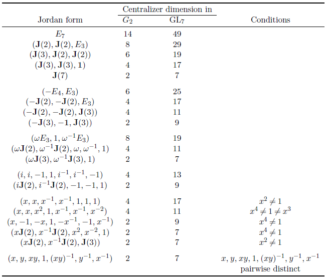
So  , hence
  . When
  , then the four centralizer adds to dimension 100. We look at the table again and there are only the following three cases
 ,
, ,
, .
.
We can rule out all these three cases due to the necessary criterion for irreducibility:  . Namely, the Euler characteristic formula tells us that
  or
or  For example, case is ruled out because then the Jordan form is
  by the table: if we twist by the character with local monodromies
  at the three finite points (and at ), we then get a new local system with local monodromies
  , which violates the above irreducible criterion. Other cases are similar.
Now  . Again the cohomological rigidity implies that the sum of dimensions of the three centralizers is 51. The table implies that the possibilities are
 ,
, ,
, ,
, ,
, ,
, ,
, .
.
The necessary criterion of irreducibility implies that  . This excludes the cases a), d), e), g). Since the monodromy group is assumed to be all of (so far we only used the monodromy group is contained in ), the (14 dimensional) adjoint representation of
  is also irreducible (the adjoint representation is irreducible for general simple reductive groups). Applying the irreducibility criterion gives
  So the sum of dimensions of the three centralizers in is less than 14. This excludes the cases b), f). The corresponding centralizers for case c) must be
  . The local monodromies are
- at ,
 at ,
at ,- several possibilities at .
The first part the follows by checking which of these possibilities can arise using Katz's algorithm.
For example, take the case at the third point . Write  for the rank 1 local system with local monodromies
  at and
  at . Twisting by
  we get ,
  and
and  . Then the rank formula together with the table tells us that the rank of the middle convolution
  is equal to
  , with local monodromies
  ,
,  ,
,  . Twisting by
  and take middle convolution, we obtain local monodromies
  ,
,  ,
,  (rank 5),... until we get down to , , (rank 2) and
  (rank 1). The last rank 1 local system actually exists since
  . Now running the algorithm reversely proves that the original local system also exists.
The final thing to do is to prove the monodromy group is actually . First notice that our monodromy representation is orthogonal. The dual representation has the same local monodromies (up to -conjugacy); since is physically rigid, this implies that  . Since the dimension 7 is odd, must be orthogonal. So maps into
  .
.
We use the fact that an irreducible subgroup of lies inside an  -conjugate of
  if and only if
  . So we need to show that
  , i.e.,
  . By the Poincare duality, this is equivalent to
  . We compute the Euler characteristic,
- At : the is the image of of in
 via the 6-th symmetric power
  Since
Since  is the same as the number of irreducible constituents of this -representation, we know
  .
. - At : the local monodromy is semisimple and it is easy to see that the dimension
 (either two 's or no 's).
 - At : the local monodromy is the image of of via
 . The number of irreducible constituents of
  is 13.
So the Euler characteristic is  . Hence
  . Therefore our lands inside . The fact (going back to Dynkin) is that an irreducible subgroup of containing a regular unipotent element must be either or . The rules out the possibility of .
□
. Therefore our lands inside . The fact (going back to Dynkin) is that an irreducible subgroup of containing a regular unipotent element must be either or . The rules out the possibility of .
□
Remark 59
One reason that the same realization of  is harder: an irreducible subgroup of containing a regular unipotent element can be
  . Another special feature about is that these rank 7 rigid local systems are also rigid when viewed as -local systems (via the adjoint representation).
is harder: an irreducible subgroup of containing a regular unipotent element can be . Another special feature about is that these rank 7 rigid local systems are also rigid when viewed as -local systems (via the adjoint representation).
04/17/2014
Remark 60
We wrap up with group theoretic consideration of the conjugacy classes of . In particular, we explain why the three conjugacy classes constructed as local monodromies actually lies inside .
. In particular, we explain why the three conjugacy classes constructed as local monodromies actually lies inside .
Take a basis of simple roots  . So
. So  (simply-connected and adjoint). Take the dual basis
  , so
, so  . The fundamental weights are
  and
and  . Using fact that
  (
( are fundamental weights), one can find
  ,
,  . The 7-dimension representation
  has weights
  (the nonzero weights form a single Weyl orbit, so it is quasi-minuscule).
The semisimple case is easy:  gives the torus
  . Taking
  gives exactly
  .
.
is the regular nilpotent orbit (the unique maximal nilpotent orbit) in  . In general
  does not necessarily take regular nilpotents to regular nilpotents, but this is the case for
  . In fact, to compute where the principle -triple
  in
in  goes in
  , just compute the pairings
  (since
  for any simple root ). It follows that the composite
  is the 6-th symmetric power, hence maps to the regular nilpotent class.
The last case is  . To any subset
  , let
, let  be the corresponding parabolic
  . For , we have two parabolic subgroups
  . Each
  has Levi subgroup
  with semisimple part a . To compute the image of the regular nilpotent in
  , just to compute
  , which is
  for
for  . So the composite is the map
  as desired. (Similar, it gives
  when
when  .)
.)
Universal rigid local systems
Let be an algebraically closed field,  . Fix an order of quasi-unipotence
  (
( ) and fix
  a primitive -th root of unity.
Let  and
and  be a cohomologically rigid local system, lisse on
  with eigenvalues contained in
  . We will show how to produce a local system over the arithmetic configuration space of points, whose geometric fibers over
  are cohomologically rigid objects in
  lisse away from and one of which gives the original
  .
.
![$R_{N,\ell}=\mathbb{Z}[\zeta_N,1/N \ell]$](./latex/latex2png-PureMotives_260666949_-5.gif) and fix a nonzero map
and fix a nonzero map  . The configuration space over
  is defined to be (
 of)
of) ![$$S_{N,n,\ell}=R_{N,\ell}[T_1,\ldots, T_n][1/\prod_{i\ne j}(T_i-T_j)].$$](./latex/latex2png-PureMotives_91745544_.gif)
The universal rigid local system will live on  , i.e.,
 ![$$\Spec R_{N,\ell}[T_1,\ldots,T_n,X][1/\prod(T_i-T_j)\prod(X-T_i)].$$](./latex/latex2png-PureMotives_200526770_.gif) Notice that one can specialize to via
Notice that one can specialize to via  .
.
Theorem 24
Fix  (inducing
  ).
).
(inducing ).
- There exists a lisse
 -sheaf on , which, after specializing along
  , recovers
  .
. - Let
 . The restriction of to any geometric fiber is a cohomologically rigid object in the corresponding category (i.e., specialization preserves index of rigidity, tameness, irreducibility, and in some sense preserves the local monodromies as ).
 - is pure of some integer weight. The characteristic polynomials of the Frobenius (when specializing to a finite field) lies in
![$\mathbb{Z}[\mu_N]$](./latex/latex2png-PureMotives_160451808_-5.gif) .
. - For any other prime
 and
and ![$\lambda': \mathbb{Z}[\mu_N]\hookrightarrow \overline{\mathbb{Q}_\ell}$](./latex/latex2png-PureMotives_182890741_-5.gif) . There exists a lisse
. There exists a lisse  -sheaf
  on
on  satisfying for any
  , the characteristic polynomials of
  on is equal to the characteristic polynomial of on
  in . In other words, we get a compatible system of -adic representations.
Proof
We will need to make sense of middle convolution in this relative setting to run Katz's algorithm. Admitting that there is a well-behaved notion of middle convolution on  for some reasonable ring (e.g,
  ), we can induct on
  .
.
for some reasonable ring (e.g, ), we can induct on .
When  . Let
. Let  be the local monodromy character, of order dividing
  ; so
; so  . Now we can spread this out by interpreting
  as associated to
  a Galois covering with Galois group
  . From the fixed map
  , we can identify
  , so we can view
  as a character of the Galois group of the covering
  In this way we obtain a lisse sheaf
  on
on  . Then
  works.
By Katz's algorithm, we can find  of rank 1 lisse on and a nontrivial character such that
  has rank strictly smaller than . We can now again spread to as above and by induction we can spread out
  to . Now invoke the middle convolution with parameters
 ![$$\mathcal{F}=\mathcal{L}^{-1} \otimes j^*(j_*\mathcal{G}[ 1 ]*_\mathrm{mid} j_{0,*}\mathcal{L}_\chi[ 1 ])$$](./latex/latex2png-PureMotives_58922509_.gif) is what we are looking for, where
is what we are looking for, where  . In the next section, we will make sense of
  in a way that commutes with base change to and for
  specializes to the old notion of middle convolution.
□
specializes to the old notion of middle convolution.
□
04/22/2014
Middle convolution with parameters
Let be a normal domain, finite type over . Let  be a divisor given by the equation
  , where
  are all distinct. Let
  be another divisor given by
  .
.
 ,
,  -hyperplanes, given by
  ;
;  .
.
The middle convolution is an operation  where
where  is given by
  . For the application,
  since
since  .
.
![$$\mathbb{A}(2)=\Spec R[X_1,X_2][1/g_D(X_1)g_{D*D'}(X_2)g_{D'}(X_2-X_1)].$$](./latex/latex2png-PureMotives_11529045_.gif)
Then we have the following diagram ![$$\xymatrix{ & \mathbb{A}(2) \ar[ld]_{\pr_1} \ar[d]^{d} \ar[rd]^{\pr_2}& \\ \mathbb{A}^1_R-D & \mathbb{A}_R^1-D' & \mathbb{A}_R^1-D*D'},$$](./latex/latex2png-PureMotives_26671764_.gif) where
where  are the projections and is the difference morphism.
We denote  . Then the compactified projection
  is proper smooth.
 ,
,  , we define the middle convolution
  and the naive convolution
Proposition 13
Assume either that everything is tame or has a generic point of characteristic 0.
has a generic point of characteristic 0.
 and
and  are lisse and tame.
- Assume is pure of weight and
 is pure of weight
  . Then is mixed of weights
  ; is pure of weight
  . Even better, the middle convolution
  the top graded piece in the weight filtration of the naive convolution.
 - Assume or is geometrically irreducible and nonconstant. Write
 for short. Then
  unless
  .
.
Proof (Ideas of the proof)
a. Let us take  . Then
  is the complement of hyperplanes in the
  and
and  directions and the diagonal. Recall that
  is the sheaf associated to
  . Since the projection
  is trivialized with respect to the stratification
  , it can be computed as
  . It follows that the middle convolution is lisse. For a formal proof, see Katz, Sommes exponentielles, Section 4.7.
b. Recall that if is an -sheaf on (a scheme of finite type over ), we say that is pure of weight  if for any closed points
  ,
,  is pure of weight in the familiar sense. We say is mixed if it admits a filtration by subsheaves such that
  are all pure.
Theorem 25 (Weil II)
Suppose is a morphism of schemes of finite type over ( is invertible on  ). If is mixed of weight
  on then
  is mixed of weight
  .
.
is a morphism of schemes of finite type over ( is invertible on ). If is mixed of weight on then is mixed of weight .
It follows that the naive convolution is mixed of weight . The purity of the middle convolution follows from the analogous statement for curves over finite fields:
 is pure of weight
  .
.
This result is less surprising by noticing that  (the source is mixed of weight
  and the target is mixed of weight
  ). To show the graded piece statement, we use the short exact sequence of sheaves
  which gives a long exact sequence
  The last term is zero since
  is punctual. Since
  is an open immersion, we know that
  has weights
  by 1.8.9 in Weil II. So we are done since
  -term is mixed of weight .
c. We prove the ! version. We can check on geometric fibers and it suffices to show for  . Notice that
  is lisse on
  and
and  is the coinvariants under the local monodromy at . In our case,
  is unramified along
  , but
, but  is indeed ramified, and hence the coinvariants is 0.
□
is indeed ramified, and hence the coinvariants is 0.
□
Remark 62
We claim that Definition 46 does recover the old definition of the middle convolution (Definition 41) when is an algebraically closed field. This finalizes the description of the middle convolution algorithm in the universal context: it produces local systems on  that specializes to cohomologically rigid tame irreducible local systems on
  for algebraically closed.
is an algebraically closed field. This finalizes the description of the middle convolution algorithm in the universal context: it produces local systems on that specializes to cohomologically rigid tame irreducible local systems on for algebraically closed.
Notice by definition  where
where ![$K=j_{D,*}\mathcal{F}[ 1 ]$](./latex/latex2png-PureMotives_63115494_-5.gif) and
and ![$K_\chi=j_{0,*}\mathcal{L}_\chi[ 1 ]$](./latex/latex2png-PureMotives_228181477_-5.gif) . Since one can replace
. Since one can replace  by (Example 26) and hence the claim follows from
  This is a special case of the following theorem (take
  ,
,  ,
,  ).
).
Theorem 27
Suppose  is affine open, is separated finite type of an algebraically closed field .
  is proper and
  is finite. Suppose
  such that
  and are perverse. Then
  in
in  .
.
is affine open, is separated finite type of an algebraically closed field . is proper and is finite. Suppose such that and are perverse. Then in .
Proof
We have two exact sequences in , 
 The kernel and cokernel are supported on , applying
  , we obtain two distinguished triangle on , four out of the six terms are perverse by assumption. One can check that
  is perverse by taking the long exact sequence on cohomology, hence the two distinguished triangles are indeed short exact sequences of perverse sheaves. Splicing together we obtain the result.
□
is perverse by taking the long exact sequence on cohomology, hence the two distinguished triangles are indeed short exact sequences of perverse sheaves. Splicing together we obtain the result.
□
, The kernel and cokernel are supported on , applying , we obtain two distinguished triangle on , four out of the six terms are perverse by assumption. One can check that is perverse by taking the long exact sequence on cohomology, hence the two distinguished triangles are indeed short exact sequences of perverse sheaves. Splicing together we obtain the result.
□
 with a finite group
 ![$e\in \overline{\mathbb{Q}_\ell}[\Gamma]$](./latex/latex2png-PureMotives_263888349_-5.gif) such that
such that  Moreover, for any
  ,
,  .
.