There are expanded notes prepared for a talk in a learning seminar on Fargues' UChicago notes Geometrization of the local Langlands correspondence, January 2016 at Columbia. Our main goal is to state the classification theorem of vector bundles on the Fargues-Fontaine curve and give a sketch of the proof. To put things in context, we first review the moduli space of vector bundles on curves and discuss the analogy between the Fargues-Fontaine curve and  .
.
[-] Contents
 Review: vector bundles on curves
Let  be a smooth projective curve. There is a nice moduli space parameterizing isomorphism classes of line bundles on
  , its the Picard variety. Unlike the case of line bundles, isomorphism classes vector bundles of higher rank in general do not form nice moduli space, e.g., the jump phenomenon shows that it is not even separated. To resolve this issue, one can either remove the word "isomorphism classes'' and work directly with the moduli stack of vector bundles
  . Or more concretely, restrict one's attention to those vector bundles which are semi-stable and construct a nice moduli space of semi-stable vector bundles using Mumford's GIT. The latter coincides with the coarse moduli space of the open substack of consisting of semi-stable vector bundles.
We briefly recall the notion of (semi-)stability and the Harder-Narasimhan filtration.
Definition 1
The slope of a vector bundle  on is the ratio
  . If we draw the vector
  in the plane then
  is literally its slope. Since both the degree and the rank are additive in a short exact sequence, we know the three vectors in an extension satisfy the parallel rule. In particular, if
  is a subbundle, then is squeezed between
  and
and  .
.
on is the ratio . If we draw the vector in the plane then is literally its slope. Since both the degree and the rank are additive in a short exact sequence, we know the three vectors in an extension satisfy the parallel rule. In particular, if is a subbundle, then is squeezed between and .
Definition 2
We say a vector bundle is stable (resp. semi-stable) if its slope is strictly bigger (resp. bigger) than that of any of its proper subbundle. Equivalently, by the squeeze property, is stable (resp. semi-stable) if its slope is strictly smaller (resp. smaller) than that of any of its proper quotient bundle. By definition any line bundle is stable.
is stable (resp. semi-stable) if its slope is strictly bigger (resp. bigger) than that of any of its proper subbundle. Equivalently, by the squeeze property, is stable (resp. semi-stable) if its slope is strictly smaller (resp. smaller) than that of any of its proper quotient bundle. By definition any line bundle is stable.
The following facts are not so difficult to prove:
Theorem 1
- The category
 of semi-stable bundles of a fixed slope
  is an abelian category: in particular, kernels and cokernels are still semi-stable bundles with the same slope.
 - For any semi-stable bundle , there is a Jordan-Holder filtration
 , such that each successive quotient is stable (necessarily of the same slope by the first part). In particular, the simple objects of are the stable bundles.
 - For any vector bundle , there is a unique filtration, known as the Harder-Narasimhan filtration or the slope filtration
 such that the successive quotients are all semi-stable with slopes strictly increasing:
  . (The construction starts off: pick the maximal subbundle
  among all subbunldes of maximal slope)
Let us look at the case  to illustrate these notions.
Example 1
By Grothendieck's theorem, each vector bundle on is a direct sum of line bundles. It follows that
is a direct sum of line bundles. It follows that
- The only stable bundles are line bundles. Every semi-stable bundle has integer slope
 and is a direct sum of
  .
. - The Harder-Narasimhan filtration of any vector bundle is split.
- The map
 gives a bijection between integral sequences
  and
and 
Remark 1
The Narasimhan-Seshadri theorem asserts that there is an equivalence between the category of semi-stable holomorphic vector bundles of slope zero on a Riemann surface and the category of unitary representations of  . As the simple objects, the stable vector bundles correspond exactly to the irreducible representations. For , the category of representations of
  indexed by integers
  , which correspond to the trivial vector bundles
  . Donaldson gives a conceptual proof of Narasimhan-Seshadri theorem by constructing a flat unitary connection on such vector bundles and the corresponding unitary representation is its monodromy representation.
and the category of unitary representations of . As the simple objects, the stable vector bundles correspond exactly to the irreducible representations. For , the category of representations of indexed by integers , which correspond to the trivial vector bundles . Donaldson gives a conceptual proof of Narasimhan-Seshadri theorem by constructing a flat unitary connection on such vector bundles and the corresponding unitary representation is its monodromy representation.
We will see soon that the classification of vector bundles on the Fargues-Fontaine curve remarkably resembles that of (and one may even think the Fargues-Fontaine curve as a "twisted "!).
The Fargues-Fontaine curve is like , but not quite
Let be a discretely valued non-archimedean field with uniformizer  and residue field
  . Let
. Let  be a perfectoid field with uniformizer
  . We have constructed the Fargues-Fontaine curve (a.k.a. the fundamental curve of
  -adic Hodge theory)
  . Recall:
 is the unique -adically complete -torsion free lift of
  as an -algebra. Concretely,
  if
if  and
and ![$\mathbb{A}=\mathcal{O}_F[ [\pi] ]$](./latex/FarguesFontaine/latex2png-FarguesFontaine_91410351_-5.gif) if
if  .
.![$Y=\Spa(\mathbb{A})-V(\pi[\varpi_F])$](./latex/FarguesFontaine/latex2png-FarguesFontaine_85878115_-5.gif) , where
, where ![$[\varpi_F]\in \mathbb{A}$](./latex/FarguesFontaine/latex2png-FarguesFontaine_168700019_-5.gif) is the Teichmuller lift. This is an adic space: the structure presheaf is actually a sheaf, thanks to Scholze.
is the Teichmuller lift. This is an adic space: the structure presheaf is actually a sheaf, thanks to Scholze. is a Frechet algebra given by the completion of
 ![$\mathbb{A}[1/\pi, 1/[\varpi_F]]$](./latex/FarguesFontaine/latex2png-FarguesFontaine_164648887_-5.gif) with respect to a family of norms indexed by compact intervals in
with respect to a family of norms indexed by compact intervals in  . The ring
  can be thought of (as least in the equal characteristic case) as holomorphic functions on the punctured open unit disk (with variable and coefficient in
  ).
).- Let
 acts
acts  by the (lift of) Frobenius on . The action is properly discontinuous and so the quotient
  makes sense and becomes an adic space over .
Remark 2
The role of the perfectoid field can be thought of as a test scheme over an absolute base " ", for the curve "
 ". So
". So  can be thought of as "
 ".
".
can be thought of as a test scheme over an absolute base "", for the curve "". So can be thought of as "".
Remark 3
It turns out that the coverings  when
when  ,
,  vary over finite extensions form a universal covering and hence its arithmetic etale fundamental
  and its geometric etale fundamental group
  . Thus the following can be thought of as an analogue of Narasimhan-Seshadri theorem: there is an equivalence between the category of semi-stable vector bundles of slope 0 on and the category of
  -representations over .
when , vary over finite extensions form a universal covering and hence its arithmetic etale fundamental and its geometric etale fundamental group . Thus the following can be thought of as an analogue of Narasimhan-Seshadri theorem: there is an equivalence between the category of semi-stable vector bundles of slope 0 on and the category of -representations over .
For any integer , we constructed the line bundle on . Geometrically it is given by  , where acts on
  by
by  . Its global section is then given by
  . We defined the schematic curve
 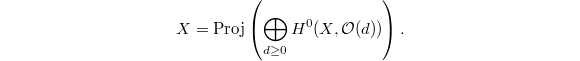 It is a scheme over , noetherian, regular, dimensional one but not of finite type.
From now on assume is algebraically closed. Let us see the first resemblance of to by computing the Picard group of . We claim that the degree map gives an isomorphism  In fact, let
  be a section whose divisor is a closed point
  . Then
 ![$$X-\{\infty_t\}=\Spec B[1/t]^{\phi=\Id}.$$](./latex/FarguesFontaine/latex2png-FarguesFontaine_236105797_.gif) It turns out (requires some work) that
It turns out (requires some work) that ![$B_e:=B[1/t]^{\phi=\Id}$](./latex/FarguesFontaine/latex2png-FarguesFontaine_247481642_-5.gif) is a PID. It then follows that
is a PID. It then follows that 
 has divisor
  and
and ![$\mathbb{P}^1-\{\infty\}=\Spec k[x]$](./latex/FarguesFontaine/latex2png-FarguesFontaine_164275513_-5.gif) is a PID and hence
is a PID and hence  .
.
Remark 5
In fact  is almost Euclidean for the degree function
  . Namely for any two nontrivial elements
  , there exists
  such that
  Notice Euclidean means that the strict inequality
  holds.
is almost Euclidean for the degree function . Namely for any two nontrivial elements , there exists such that Notice Euclidean means that the strict inequality holds.
Let us see another resemblance to by showing the "genus" of is zero, i.e.,  . We have an affine covering
  and
and  an infinitesimal neighborhood of
  . The cohomology of coherent sheaf
  on can be computed by the Cech complex
  Namely
  For
For  , since
  and
and ![$\mathcal{O}_X(U_1\cap U_2)=B_\mathrm{dR}:=B_\mathrm{dR}[1/t]$](./latex/FarguesFontaine/latex2png-FarguesFontaine_64022799_-5.gif) , it reads
, it reads  The latter has to do with the fact that is almost Euclidean.
Remark 6
Warning: however, fails to satisfy Riemann-Roch:  which has to do with the fact that is not Euclidean. This is the main difference causing the classification of vector bundles on to be more complicated than the case of .
fails to satisfy Riemann-Roch: which has to do with the fact that is not Euclidean. This is the main difference causing the classification of vector bundles on to be more complicated than the case of .
Vector bundles on the Fargues-Fontaine curve
Let  be the degree unramified extension. Notice if we replace by
  then stays the same but the Frobenius changes since the residue field of changes. Thus we have a natural degree unramified cover
Definition 3
We can push forward the line bundle  along
along  to get a vector bundle
  of rank and degree . Its slope is
  . We denote it by
  when
when  .
.
along to get a vector bundle of rank and degree . Its slope is . We denote it by when .
We have following easy properties analogous to the case:
Proposition 1
 .
. if and only
  . In particular,
  if and only
  .
. if
if  . In particular, by (a), there is no nontrivial extension of by
  if
if  .
.
Now we can state the main classification theorem.
Theorem 2
Suppose is algebraically closed.
is algebraically closed.
- The semi-stable stable vector bundles of slope are direct sums of .
- The Harder-Narasimhan filtration of any vector bundle on is split.
- The map
 gives a bijection between sequences
  (
( ) and
) and 
Notice (a) implies (b) by the third property in Proposition 1; (a,b) together implies (c).
Remark 7
In the equal characteristic, this theorem is due to Hartl-Pink's classification of -equivariant vector bundles over  . In the mixed characteristic, this theorem is equivalent to Kedlaya's classification of -modules over the Robba ring
  (by the expanding property of ). We are going to discuss a more geometric proof due to Fargues.
-equivariant vector bundles over . In the mixed characteristic, this theorem is equivalent to Kedlaya's classification of -modules over the Robba ring (by the expanding property of ). We are going to discuss a more geometric proof due to Fargues.
Remark 8
This classification may remind you the Dieudonne-Manin classification of isocrystals. In fact, let  and let
  be an isocrystal over
  . Then the vector bundle corresponding to
  (the minus sign comes from normalization) can be realized geometrically as
  !
!
and let be an isocrystal over . Then the vector bundle corresponding to (the minus sign comes from normalization) can be realized geometrically as !
Reduction to degree one modifications of vector bundles
The main goal today is to reduce to the classification theorem 2 to the following two statements about modification of vector bundles on the Fargues-Fontaine curve.
Theorem 3
- If
 is an increasing modification of of degree one, i.e., there is an exact sequence
  with
with  for a closed point
  , then
  .
. - If is an increasing modification of of degree one,
 then
then  for some
  .
.
Remark 9
The modifications of a vector bundle at are given by specifying a lattice in  , where is the isocrystal with the same slopes as . Moreover, the degree one modification are given by the lattices satisfying the minuscule condition. Then Theorem 3 are proved by showing that all lattices corresponding to the desired modification can be realized as the period lattices of -divisible groups, which can be explicitly described. It thus boils down to the study of period maps on certain Rapoport-Zink deformation spaces of -divisible groups. Part (a) reduces to the surjectivity of the de Rham period map from the Lubin-Tate space to
  (due to Gross-Hopkins). Part (b) reduces to that any point in Drinfeld's half space
  comes from the Hodge-Tate period of the dual of a Lubin-Tate formal group, which in turn reduces to that the image of the de Rham period of the Rapoport-Zink space of special formal
  -modules of height
  is exactly
  (due to Drinfeld).
at are given by specifying a lattice in , where is the isocrystal with the same slopes as . Moreover, the degree one modification are given by the lattices satisfying the minuscule condition. Then Theorem 3 are proved by showing that all lattices corresponding to the desired modification can be realized as the period lattices of -divisible groups, which can be explicitly described. It thus boils down to the study of period maps on certain Rapoport-Zink deformation spaces of -divisible groups. Part (a) reduces to the surjectivity of the de Rham period map from the Lubin-Tate space to (due to Gross-Hopkins). Part (b) reduces to that any point in Drinfeld's half space comes from the Hodge-Tate period of the dual of a Lubin-Tate formal group, which in turn reduces to that the image of the de Rham period of the Rapoport-Zink space of special formal -modules of height is exactly (due to Drinfeld).
Our remaining goal is show that Theorem 2 is equivalent to Theorem 3, in a spirit similar to Grothendieck's proof for . One direction is easy to verify.
Proof (Theorem 2  3)
3)
3)
- Since
 has degree 1 and rank 0, we know that has degree 0 and rank . Suppose
  , then
  by the second property. Since
  , we know that
  or
or  . But
. But  , so .
 - Similarly, we have
 and
and  . Suppose , then
  by the second property. Therefore one
  and the others are all 0.
□
and the others are all 0.
□
The other direction is harder. We reduce to the following lemma.
 is exact, then
Proof
One direction is clear since if and , then some and hence  by second property.
and , then some and hence by second property.
For the other direction, we need to show that every semi-stable vector bundle is a direct sum of . It turns out that  is semi-stable stable if and only if
  is semi-stable and is such a direct sum of if and only if
  is a direct sum
  . So we may assume that
  by pulling back along . Twisting by the line bundle we may assume . We need to show that
  .
.
Let us only consider the case  (i.e.,
  ). Let
  be the sub line bundle of maximal degree. It has degree
  since is semi-stable of degree 0. Write
  . We know that
  If
If  , then
  by the third property. If
  , then by assumption that , hence there is an injection
  , which contradicts the maximality of
  . More generally, if
  , then
  . There is an injection
  . Pullback the exact sequence we obtain a new exact sequence
  Hence by assumption
  , which gives an injection
  , i.e.
  , which contradicts the maximality of .
□
, which contradicts the maximality of .
□
Remark 10
The general case is done similarly by induction on the rank, which starts off by finding the maximal degree sub line bundle of in order to use the hypothesis when .
in order to use the hypothesis when .
Now it remains to prove that Theorem 3 implies the statement in Lemma 1.
Proof
We still focus on the rank 2 case. Suppose  We need to show that . Choose an injection
  . Then pushing out gives
  Hence
Hence  by the third property and we have
  Here is degree 2 torsion sheaf (cokernel of ). Choose a degree 1 subsheaf
  and pullback we obtain a degree one modification
  Hence
Hence  Taking dual
  and twist by
  we obtain another degree one modification
  By Theorem 3 (b) we know that either
  or
or  . In either case:
We need to show that . Choose an injection . Then pushing out gives Hence by the third property and we have Here is degree 2 torsion sheaf (cokernel of ). Choose a degree 1 subsheaf and pullback we obtain a degree one modification Hence Taking dual and twist by we obtain another degree one modification By Theorem 3 (b) we know that either or . In either case:
- We have
 Notice
  is either or
  , so .
 - We have
 By Theorem 3 (1) we know that
  , hence
  .
□
.
□
Remark 11
The general case is done similarly, which starts off by choosing an injection  to get a degree
  modification
  Then one write this as a sequence of degree one modifications and use Theorem 3 (a) or (b) at each step.
to get a degree modification Then one write this as a sequence of degree one modifications and use Theorem 3 (a) or (b) at each step.
Last Update:
04/14/2016. Copyright © 2015, Chao Li.